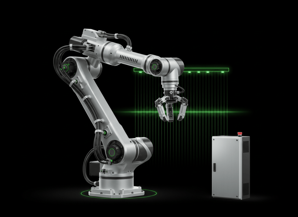
Robotics engineering begins when “move the arm there” becomes a precise mathematical question: where is “there,” relative to which frame, and what joint values place the tool at that pose?

This is OSREC.001, the first lesson in the Open Source Robotics Engineer Certification track. It builds from the technician view of robot hardware into the mathematical structure engineers use to describe and command motion.

For a shorter introduction to the topic, revisit our earlier Robot Kinematics article. This lesson goes deeper into coordinate frames, transformations, forward kinematics, inverse kinematics, and the engineering mistakes that appear when those ideas are implemented incorrectly.

The whole lesson in one flow

joint positions define robot configuration
↓
coordinate frames define where bodies are measured from
↓
transformations relate one frame to another
↓
forward kinematics maps joints → tool pose
↓
inverse kinematics maps desired tool pose → joint solution(s)
↓
trajectory generation connects poses over time
↓
control drives motors so the physical robot follows the mathematical command

1. Configuration and degrees of freedom

A robot’s configuration is the set of variables needed to describe its mechanical state. For a simple six-axis articulated arm, the configuration can usually be represented by six joint variables:

q = [q₁, q₂, q₃, q₄, q₅, q₆]

Each independent variable corresponds to one degree of freedom. Different industrial robot types arrange those degrees of freedom differently: articulated arms use rotary joints, Cartesian robots rely heavily on linear axes, SCARA robots combine planar rotary motion with vertical translation, and parallel robots use closed mechanical chains.

The geometry matters because the same desired tool motion can require very different joint motion depending on the mechanism.

Reference: Northwestern Modern Robotics — Foundations of Robot Motion.

2. Coordinate frames: every pose needs a reference

A position such as “X = 400 mm” is incomplete unless the engineer states the reference frame. Robotics uses coordinate frames to define both position and orientation.

• World frame: a fixed global reference for the workcell.
• Base frame: attached to the robot base.
• Joint/link frames: attached to robot links or joints for kinematic calculations.
• Tool frame: attached to the end effector.
• TCP frame: centered at the tool center point that matters to the task.
• Work/object frame: attached to a fixture, part, conveyor, pallet, or workpiece.
• Camera frame: attached to a vision sensor.

Two engineers can describe the same physical point with different numbers if they use different frames. The numbers differ; the physical point does not.

Video 1: Coordinate transformations

3. Position and orientation are different quantities

A robot tool pose contains both:

• Position: where the origin of the tool frame is located.
• Orientation: how the tool frame is rotated relative to the reference frame.

In three dimensions, position is commonly represented by a vector p = [x, y, z]. Orientation may be represented by a rotation matrix, Euler angles, axis-angle coordinates, or a quaternion. Each representation has advantages and failure modes.

For industrial work, orientation errors can be just as damaging as position errors. A welding torch can arrive at the correct XYZ location but still be unusable if its approach angle is wrong.

4. Homogeneous transformations

A homogeneous transformation combines rotation and translation into one mathematical object. In compact block form:

T = [ R  p ; 0  1 ]

Here R describes orientation and p describes translation. Transformations can be multiplied to chain frames together.

For example:

world → robot base
robot base → wrist
wrist → tool
tool → TCP

Multiplying the appropriate transforms lets the engineer express the TCP pose in the world frame.

MathWorks documents the same family of robotics representations through rotation matrices, quaternions, and SE(3) homogeneous transformations: Coordinate Transformations — MATLAB & Simulink.

5. Forward kinematics: joints to tool pose

Forward kinematics answers:

Given the joint values, where is the end effector?

Mathematically, the relationship can be written as:

x = f(q)

where q is the joint configuration and x is the resulting tool pose.

Forward kinematics is usually deterministic: for a given valid joint configuration, the robot has one physical pose. Different formulations can be used to derive it, including Denavit–Hartenberg parameters or product-of-exponentials methods.

Northwestern’s Modern Robotics Chapter 4 treats forward kinematics explicitly in the space and end-effector frames: Modern Robotics — Chapter 4.

Video 2: Forward kinematics

6. Inverse kinematics: desired pose to joints

Inverse kinematics asks the reverse question:

What joint values place the end effector at this desired pose?

Conceptually:

q = f⁻¹(x)

But unlike simple scalar inversion, robot inverse kinematics may have:

• no solution because the pose is outside the workspace;
• one solution;
• multiple valid joint solutions;
• infinitely many solutions in redundant robots;
• numerically unstable behavior near a singularity.

For a six-axis arm, the same TCP pose may be reachable with different shoulder, elbow, or wrist configurations. Engineers must choose the solution that respects limits, collision constraints, cable routing, cycle time, and process requirements.

Reference: Modern Robotics — Chapter 6: Inverse Kinematics.

Video 3: Inverse kinematics

7. Joint space and task space

Joint space describes motion using joint variables. Task space describes motion using the end-effector pose or task variables.

A straight line in joint space generally does not produce a straight-line TCP path. Likewise, a straight Cartesian tool path usually requires nonlinear coordinated motion across several joints.

This distinction matters in welding, dispensing, machining, inspection, and any process where the path of the tool—not merely the final pose—must be controlled.

8. The tool center point

The tool center point (TCP) is the task-relevant point attached to the end effector. It may be the center of a gripper, welding wire tip, screwdriver bit, camera optical reference, or dispensing nozzle.

A robot can have perfectly healthy drive systems and still miss the part if the TCP definition is wrong.

Common causes of TCP error include:

• tool replaced without recalibration;
• tool bent after a collision;
• incorrect tool length entered;
• wrong active tool frame;
• end-effector fixture shifted;
• payload or center-of-gravity data entered incorrectly.

9. Kinematic models assume real mechanics behave

The mathematical model assumes the physical joints and links match the modeled geometry. Real mechanisms introduce error through compliance, backlash, bearing play, calibration offsets, thermal expansion, and reducer error.

This is where robot math meets mechanical design. Earlier BitcoinVersus lessons on gear trains and reducers and displacement measurement matter directly to robotics engineering because the control model is only as good as the mechanical transmission and feedback data.

10. Singularities

A kinematic singularity is a robot configuration where the mapping between joint motion and Cartesian motion loses rank. Practically, the robot can lose the ability to move the tool freely in one or more directions, or a small desired Cartesian velocity may require very large joint velocities.

Symptoms can include:

• unexpected wrist speed near certain poses;
• motion planner refusing a path;
• joint velocities increasing sharply;
• orientation flipping to another inverse-kinematics branch;
• poor numerical convergence.

Singularities are not simply software bugs. They arise from robot geometry.

11. Coordinate frames in robotics software

Modern industrial robotics software stacks maintain relationships among many moving frames: world, base, links, cameras, tools, parts, and targets. The math is the same whether the transform comes from a hand-derived model, a robot controller, a simulation environment, or middleware.

MathWorks’ Robotics System Toolbox similarly treats manipulators through rigid-body-tree models and includes forward/inverse kinematics, collision checking, path planning, trajectory generation, and dynamics: MathWorks — Robot Modeling.

12. Engineering troubleshooting: pose error

Suppose the robot reaches the correct general area but the tool is consistently 8 mm too high.

1. Confirm the active coordinate frame. Is the program using world, base, work-object, or tool coordinates?
2. Confirm the TCP. Was the tool changed or bent?
3. Check calibration. Are joint zero offsets valid?
4. Check fixture coordinates. Did the workpiece move?
5. Check feedback. Are joint encoders and external measurement systems consistent?
6. Check mechanics. Is there backlash, looseness, or reducer damage?
7. Check the model. Are link lengths, offsets, and frame transforms correct?

Do not immediately retouch every programmed point. If one frame or TCP is wrong, changing dozens of points can hide the root cause and make the system harder to restore.

13. Engineering troubleshooting: wrong inverse-kinematics branch

Suppose the tool reaches the same target pose but the elbow swings to the opposite side of the machine.

The target may have multiple valid IK solutions. The engineering task is to apply constraints or choose a seed/configuration that selects the intended shoulder, elbow, and wrist branch.

• respect joint limits;
• avoid collisions;
• avoid singularities;
• minimize unnecessary joint travel;
• keep cables and hoses within safe routing;
• preserve process orientation.

14. Practice exercise

A six-axis robot has a camera mounted above the workcell. The camera reports a part position in the camera frame, but the robot controller commands motion in the base frame.

Think through the chain:

camera measurement
↓
camera-to-world calibration
↓
world-to-base transform
↓
desired TCP pose in base coordinates
↓
inverse kinematics
↓
joint target

If the camera calibration is wrong by 5 mm, the inverse kinematics may be mathematically perfect and the robot can still miss the part by about 5 mm. Good mathematics cannot correct bad frame calibration.

Knowledge check

1. What does forward kinematics compute?
The end-effector pose from known joint values.

2. What does inverse kinematics compute?
One or more joint configurations that can produce a desired end-effector pose.

3. Why are coordinate frames necessary?
Because position and orientation only have meaning relative to a defined reference.

4. What is a TCP?
The task-relevant point and frame attached to the robot’s tool.

5. Why can inverse kinematics have multiple answers?
Because different joint configurations can place the same end effector at the same pose.

6. What is a singularity?
A configuration where the robot loses independent Cartesian motion capability because the joint-to-task-space mapping becomes rank deficient.

7. Why can a robot with healthy motors still miss a target?
Because frame calibration, TCP data, fixture coordinates, mechanical geometry, or feedback can be wrong even when the actuators work correctly.

Key takeaway

Robot motion is geometry expressed through coordinate frames. Forward kinematics tells an engineer where the tool goes when the joints move. Inverse kinematics tells the engineer which joints can produce a desired tool pose. Transformations connect frames. Calibration connects the mathematics to the real machine. Once those foundations are solid, trajectory planning, dynamics, control, perception, and autonomous manipulation become much easier to reason about.

Display note: all formulas and motion flows in this lesson are educational text, not terminal simulations. No Windows, Linux, or VS Code terminal colors are represented or invented.

BitcoinVersus.Tech

Advertisement

Use the #promocode bitcoinversus at check out to Get 5% off #Bitaxe Mining Products

Limited to one use per customer Happy #Bitcoin Mining!https://t.co/0trBgXkbVd

— BitcoinVersus.Tech 📟 (@1BitcoinVersus) June 23, 2025

Editor’s Note:

We volunteer daily to ensure the credibility of the information on this platform is Verifiably True. If you would like to support our research initiatives, please donate here: 3C9o19EH5HSiwEPyCTmEKzxhNCbo2X6TTb

BitcoinVersus.tech is not a financial advisor. This media platform reports on financial subjects purely for informational purposes.