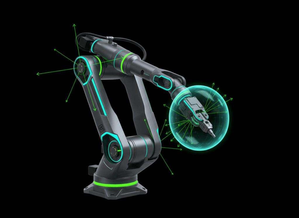
A robot Jacobian converts motion in joint space into instantaneous motion at the end effector. It is the local mathematical bridge between actuator rates and task-space velocity, and it is one of the central tools of robotics engineering.

OSREC.002 continues the Robotics Engineer sequence from OSREC.001: Robot Kinematics and Coordinate Frames — Forward and Inverse Kinematics. OSREC.001 mapped joint positions to tool pose. This lesson differentiates that relationship to study joint velocity, end-effector velocity, singularities, redundancy, manipulability, and differential inverse kinematics. The technician-side manual-motion foundation appears in OSRTC.002: Teach Pendant Basics — Jogging, Coordinate Frames, Speed, and Safe Manual Positioning.

The Jacobian in one equation

For a robot with joint coordinates q and joint rates q̇, the end-effector twist or task-space velocity can be written:

V = J(q) q̇

• V = end-effector linear and angular velocity representation
• J(q) = Jacobian evaluated at the current robot configuration
• q̇ = vector of joint velocities

The important feature is that J depends on configuration. A robot can have the same motors, links, and controller while the instantaneous relationship between joint motion and tool motion changes continuously as the arm moves.

Northwestern University’s Modern Robotics Chapter 5 — Velocity Kinematics and Statics develops this exact progression from forward kinematics to Jacobians, singularities, statics, and manipulability.

Video 1: Velocity kinematics and statics

1. From forward kinematics to velocity kinematics

Forward kinematics represents tool pose as a function of joint position:

x = f(q)

Differentiating with respect to time gives the local velocity relationship:

ẋ = J(q)q̇

For a simple Cartesian coordinate representation, each Jacobian column describes how one joint contributes to the instantaneous end-effector velocity. In three-dimensional rigid-body robotics, the velocity representation is commonly a six-component twist containing angular and linear velocity.

2. Jacobian columns are motion contributions

Consider an n-joint robot. Its Jacobian contains n columns:

J = [J₁ J₂ … Jₙ]

The resulting tool velocity is the weighted sum:

V = J₁q̇₁ + J₂q̇₂ + … + Jₙq̇ₙ

This interpretation is useful because each column describes the instantaneous motion direction produced by one unit of velocity at one joint while the configuration is held fixed.

3. Revolute and prismatic joints contribute differently

A revolute joint contributes angular velocity and corresponding linear velocity at the tool because the tool rotates about that joint axis. A prismatic joint contributes translational velocity along its axis.

• Revolute joint: rotational joint rate produces both angular and position-dependent linear tool motion.
• Prismatic joint: linear joint rate contributes translation along the prismatic axis.

This is why Jacobian construction depends on the robot’s kinematic architecture, not merely on the number of joints.

4. Space Jacobian and body Jacobian

The same physical end-effector motion can be expressed in different coordinate frames. Two common formulations are:

• Space Jacobian J_s: maps joint rates to the end-effector twist expressed in the fixed space frame.
• Body Jacobian J_b: maps joint rates to the end-effector twist expressed in the end-effector or body frame.

The physical motion is the same; the numerical velocity coordinates differ because the reference frame differs. Frame discipline from OSREC.001 therefore remains essential.

Video 2: Space Jacobian

5. Two-link planar arm example

For a planar two-revolute-joint arm with link lengths l₁ and l₂:

x = l₁ cos q₁ + l₂ cos(q₁ + q₂)
y = l₁ sin q₁ + l₂ sin(q₁ + q₂)

Differentiating gives:

[ẋ ẏ]ᵀ = J(q)[q̇₁ q̇₂]ᵀ

with:

J(q) =
[−l₁ sin q₁ − l₂ sin(q₁+q₂), −l₂ sin(q₁+q₂)]
[ l₁ cos q₁ + l₂ cos(q₁+q₂), l₂ cos(q₁+q₂)]

The determinant is:

det J = l₁l₂ sin q₂

When q₂ = 0 or π, the two links are collinear and the determinant becomes zero. The Jacobian loses rank: the arm cannot generate arbitrary planar tip velocity directions at that instant.

6. Rank explains available instantaneous motion

The rank of a Jacobian measures how many independent task-space velocity directions can be produced locally.

• Full rank: the robot can generate all locally available independent velocity directions for that model.
• Rank deficient: one or more instantaneous task-space directions become unavailable.

A singularity occurs when the Jacobian loses rank relative to its normal capability. The mechanical robot may still move, but the mapping between joint and task-space velocities has lost an independent direction.

7. Singularities are configuration-dependent

Singularities are not normally caused by a broken motor or bad encoder. They are properties of the robot geometry at particular configurations.

• A stretched planar arm loses one instantaneous direction.
• A six-axis wrist can align multiple rotational axes and lose independent orientation capability.
• A shoulder or elbow geometry can reach a configuration where distinct joint effects become linearly dependent.

Northwestern’s Modern Robotics section on singularities defines the condition in terms of Jacobian rank and explicitly treats square, tall, and wide Jacobians.

Video 3: Singularities

8. Near-singular is often more important than exactly singular

Real robot controllers must manage the region near a singularity, not only the exact mathematical singular point. As the Jacobian becomes poorly conditioned, a modest desired tool velocity can require very large joint velocities.

Practical consequences include:

• large wrist or elbow rates for small TCP motion;
• velocity saturation at one or more joints;
• poor numerical behavior in differential inverse kinematics;
• path slowdown imposed by the controller;
• orientation flips or branch changes when combined with inverse kinematics;
• greater sensitivity to encoder noise and modeling error.

9. Differential inverse kinematics

Forward differential kinematics computes tool velocity from joint velocity:

V = Jq̇

Differential inverse kinematics asks the reverse question:

Given a desired instantaneous tool velocity V_d, what joint rates q̇ should be commanded?

For a square, nonsingular Jacobian:

q̇ = J⁻¹V_d

Many practical robots do not have a square invertible Jacobian at every relevant state, so robotics software commonly uses a pseudoinverse or another constrained optimization method.

10. Moore-Penrose pseudoinverse

A common least-squares differential inverse-kinematics solution is:

q̇ = J⁺V_d

where J⁺ is the Moore-Penrose pseudoinverse.

The pseudoinverse provides a principled solution when the system is redundant or overconstrained, but it does not make singularity problems disappear. Near singular configurations, the inverse of very small singular values can amplify commanded joint rates.

11. Damped least squares

A common numerical strategy near singularities is damped least squares. One form is:

q̇ = Jᵀ(JJᵀ + λ²I)⁻¹V_d

The damping term λ reduces extreme joint-rate amplification at the cost of some task-space tracking accuracy. Engineering implementation requires choosing damping intelligently rather than treating λ as an arbitrary constant.

12. Redundant robots have null-space freedom

A robot with more controllable joints than required by the primary task can have multiple joint-rate solutions that produce the same end-effector velocity.

A common form is:

q̇ = J⁺V_d + (I − J⁺J)z

The first term performs the primary tool-velocity task. The null-space term can be used for secondary objectives without changing the first-order end-effector motion.

• avoid joint limits;
• increase distance from collisions;
• improve manipulability;
• reduce energy or joint motion;
• maintain cable or hose routing;
• favor a posture for the next task.

13. Manipulability describes directional capability

The Jacobian also reveals how easily a robot can move in different task-space directions. If unit-bounded joint velocity is mapped through the Jacobian, the resulting task-space velocities form a manipulability ellipsoid.

• Long ellipsoid axes indicate directions where substantial tool velocity is comparatively easy to generate.
• Short axes indicate directions requiring more joint effort for the same tool velocity.
• An axis collapsing toward zero indicates approach to a singularity.

Manipulability is therefore a geometric measure of local motion capability, not a generic “robot quality” score.

14. Statics uses the transpose Jacobian

The Jacobian also links end-effector wrench to joint force or torque. Under the corresponding frame and sign conventions:

τ = JᵀF

• F = end-effector wrench containing force and moment components
• τ = generalized joint forces or torques

This duality explains why kinematic geometry also changes force transmission. A configuration that is favorable for velocity in one direction can have a different force capability in that direction.

15. Geometric and analytic Jacobians are not always identical

A geometric Jacobian typically maps joint rates to a spatial velocity or twist. An analytic Jacobian maps joint rates to derivatives of a chosen minimal pose-coordinate representation, such as XYZ plus Euler angles.

These can differ because orientation-coordinate derivatives are not generally identical to physical angular velocity. Euler-angle representations can also introduce representation singularities that are distinct from robot kinematic singularities.

This distinction matters in software. A singular Euler-angle parameterization does not necessarily mean the physical robot has reached a kinematic singularity.

16. Condition number as a warning metric

The singular values of J provide more information than a binary singular/not-singular test. A condition number based on the ratio between largest and smallest significant singular values indicates how uneven the velocity mapping has become.

A very large condition number means some task-space directions are becoming much harder to produce than others. Controllers and planners can use such metrics to slow motion, alter posture, add damping, or choose another path before a singularity is reached.

17. Engineering example: straight Cartesian path near a wrist singularity

Suppose a six-axis robot is commanded to maintain tool orientation while moving the TCP along a straight line. Midway through the move, two wrist axes approach alignment.

1. The desired TCP velocity remains modest.
2. The Jacobian becomes poorly conditioned.
3. The differential inverse solution demands rapidly increasing wrist-joint rates.
4. A joint-speed limit is reached.
5. The controller slows, modifies, or rejects the motion depending on its implementation.

The correct engineering diagnosis is not automatically “bad servo tuning.” The geometry must be checked first.

18. Engineering troubleshooting framework

When a robot shows unexpectedly high joint speed, poor Cartesian tracking, or numerical instability, investigate the differential kinematics systematically:

1. Verify the active robot model and joint ordering.
2. Verify coordinate-frame conventions.
3. Compute or inspect Jacobian rank and singular values.
4. Check proximity to joint limits and known singular postures.
5. Confirm whether the software uses geometric or analytic Jacobians.
6. Inspect the inverse method: direct inverse, pseudoinverse, damped least squares, or constrained optimization.
7. Check velocity and acceleration limits after the mapping into joint space.
8. Verify that the desired task-space velocity itself is physically reasonable.
9. Check the physical robot for calibration or mechanical errors only after model and configuration effects are understood.

19. Why Jacobians matter beyond industrial arms

The same differential-kinematics principles appear in many robot classes:

• humanoid arms and whole-body control;
• legged-robot foot velocity control;
• mobile manipulators;
• continuum and redundant robots;
• camera visual servoing;
• force-controlled assembly;
• teleoperation;
• inverse-kinematics solvers and motion planners;
• optimization-based control and model-predictive control.

The Jacobian is therefore not merely a matrix learned for one robotics course. It is a reusable mathematical object throughout robotics software, control, planning, and mechanical design.

Exercises

1. Starting from x = f(q), explain why differentiating produces a local linear map between q̇ and ẋ.
2. For the two-link planar arm, show why det J = l₁l₂ sin q₂ and identify the singular values of q₂ qualitatively at 0 and π.
3. Explain the physical difference between a space Jacobian and a body Jacobian.
4. Describe why a pseudoinverse can generate very large joint rates near a singularity.
5. Explain the tradeoff introduced by damped least squares.
6. List three useful secondary objectives for the null space of a redundant robot.
7. Explain why an Euler-angle representation singularity is not necessarily a robot kinematic singularity.
8. Describe how a manipulability ellipsoid changes as a robot approaches singularity.

Knowledge check

1. What does the Jacobian map?
Joint velocities to instantaneous end-effector velocity or twist at a given robot configuration.

2. Why does J depend on q?
Because each joint’s instantaneous contribution to tool motion changes with the robot’s geometry and current configuration.

3. What indicates a kinematic singularity?
The Jacobian loses rank relative to its normal capability.

4. What is differential inverse kinematics?
Computing joint rates that produce a desired instantaneous task-space velocity.

5. Why use a pseudoinverse?
It provides a least-squares or minimum-norm solution when the Jacobian is not square or when redundancy is present.

6. What does damping do near a singularity?
It reduces excessive joint-rate amplification while accepting some task-space error.

7. What is null-space motion?
Joint motion that does not change the primary end-effector velocity to first order and can be used for secondary objectives.

8. How is an end-effector wrench mapped to joint forces or torques?
Through the transpose relationship τ = JᵀF under consistent frame and sign conventions.

Key takeaway

The Jacobian is the local language of robot motion. Forward kinematics describes where the robot is; the Jacobian describes how that pose changes instantaneously. Its rank exposes singularities, its pseudoinverse enables differential inverse kinematics, its null space enables redundancy resolution, and its singular values reveal directional capability. These concepts connect geometry directly to control, planning, force transmission, and real robot behavior.

Modeling note: the equations in this lesson are introductory differential-kinematics relationships. Real controllers may add joint limits, collision constraints, dynamics, acceleration limits, filtering, task priorities, optimization, and safety-rated motion constraints.

Display note: this lesson uses standard Gutenberg paragraphs, headings, lists, and media embeds only. No decorative text-box or callout-box layout is used.

BitcoinVersus.Tech

Advertisement

Use the #promocode bitcoinversus at check out to Get 5% off #Bitaxe Mining Products

Limited to one use per customer Happy #Bitcoin Mining!https://t.co/0trBgXkbVd

— BitcoinVersus.Tech 📟 (@1BitcoinVersus) June 23, 2025

Editor’s Note:

We volunteer daily to ensure the credibility of the information on this platform is Verifiably True. If you would like to support our research initiatives, please donate here: 3C9o19EH5HSiwEPyCTmEKzxhNCbo2X6TTb

BitcoinVersus.tech is not a financial advisor. This media platform reports on financial subjects purely for informational purposes.