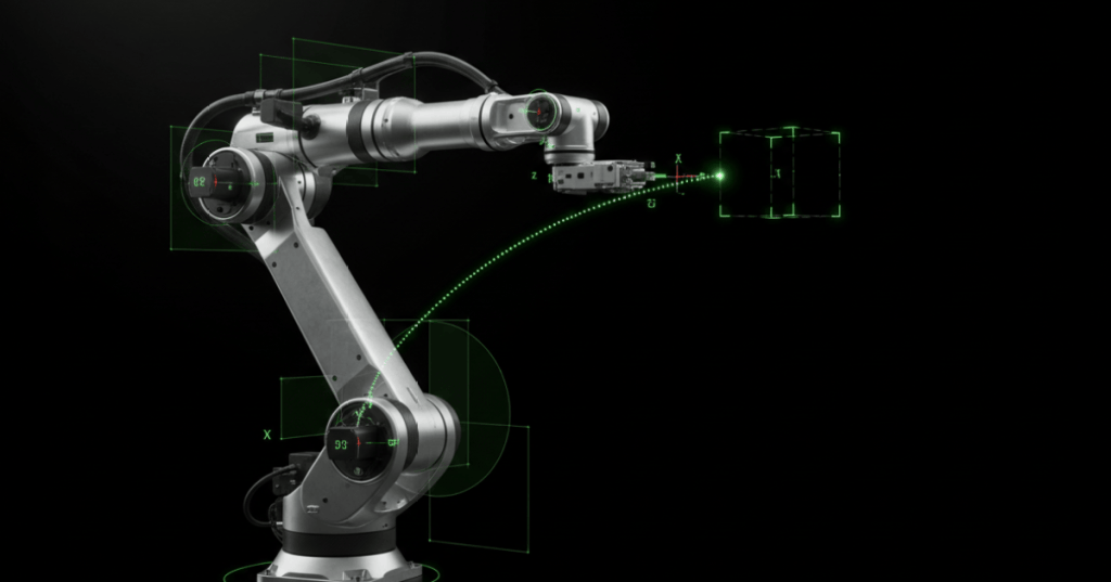
Inverse kinematics converts a desired end-effector pose into joint coordinates. Unlike forward kinematics, which maps a known joint configuration to a tool pose, inverse kinematics can have multiple solutions, no exact solution, or a solution that becomes numerically unstable near singular configurations.

OSREC.003 continues the Open Source Robotics Engineer sequence from OSREC.001: Forward Kinematics — Coordinate Frames, Transforms, and Denavit–Hartenberg Modeling and OSREC.002: Robot Jacobians — Velocity Kinematics, Singularities, and Differential Motion. It also connects directly to the practical calibration issues covered in OSRTC.003: Robot Mastering and Calibration.

The inverse-kinematics problem

Let the robot configuration be represented by the joint vector θ, and let forward kinematics be written as T(θ), where T is the end-effector pose relative to a reference frame. Inverse kinematics asks for one or more joint vectors satisfying:

T(θ) = T_d

Here T_d is the desired target pose. The target normally includes both translation and orientation. A position-only problem can be lower dimensional, but a general rigid-body pose in three-dimensional space has six task-space degrees of freedom: three translational and three rotational.

The central engineering complication is that the mapping from joint coordinates to Cartesian pose is nonlinear. Trigonometric terms, serial-link geometry, joint limits, redundant degrees of freedom, singularities, and collision constraints make inverse kinematics fundamentally different from solving a single linear matrix equation.

A solution may be unique, multiple, or nonexistent

• Unique solution: only one admissible joint configuration reaches the target under the active constraints.
• Multiple discrete solutions: several configurations reach the same pose, such as elbow-up and elbow-down solutions.
• Infinite solutions: a redundant manipulator may have a continuum of joint configurations for the same end-effector pose.
• No exact solution: the target lies outside the reachable workspace, violates orientation limits, conflicts with joint limits, or cannot be reached by the robot’s kinematic structure.
• Near-singular solution: a valid pose exists, but small Cartesian changes require very large joint changes and numerical sensitivity increases sharply.

Inverse kinematics of open chains

Analytical inverse kinematics

An analytical inverse-kinematics solution derives explicit equations for the joint variables from the desired pose. Closed-form solutions are especially valuable when the robot geometry has exploitable structure, such as intersecting wrist axes or a planar manipulator with a small number of joints.

For a simple planar two-link arm with link lengths L₁ and L₂, the end-effector position is:

x = L₁ cos θ₁ + L₂ cos(θ₁ + θ₂)

y = L₁ sin θ₁ + L₂ sin(θ₁ + θ₂)

One standard derivation first solves the elbow angle:

cos θ₂ = (x² + y² − L₁² − L₂²) / (2L₁L₂)

When the right-hand side lies between −1 and +1, two elbow branches can exist because sin θ₂ may be positive or negative. This is the classic elbow-up versus elbow-down ambiguity.

Reachability test

For the same two-link planar arm, the radial distance from the base to the target is r = √(x² + y²). A necessary geometric condition for reachability is:

|L₁ − L₂| ≤ r ≤ L₁ + L₂

A production solver should reject or project unreachable goals rather than allowing a numerical iteration to diverge indefinitely.

Why analytical solutions are attractive

• They are usually fast and deterministic.
• They can expose all discrete solution branches.
• They make geometric constraints easier to inspect.
• They can avoid iterative convergence failures.
• They are well suited to high-rate control when a closed form exists.

The limitation is generality. Arbitrary link geometry, redundancy, additional constraints, flexible mechanisms, and complex task objectives often make a clean closed-form solution impractical or impossible.

Numerical inverse kinematics

Numerical inverse kinematics starts from an initial joint estimate and iteratively reduces pose error. This makes it applicable to a much wider range of manipulators.

At iteration k, define the current configuration as θ_k. The forward-kinematics model produces the current end-effector pose. A pose-error representation is then converted into a corrective Cartesian twist or task-space error vector e_k.

The Jacobian from OSREC.002 provides the local differential relationship:

V = J(θ) θ̇

For a small iterative correction, the analogous update is:

Δθ ≈ J^† e

where J^† is an appropriate inverse, pseudoinverse, or regularized inverse of the Jacobian.

Newton–Raphson numerical inverse kinematics

Core numerical iteration

1. Choose an initial joint estimate θ₀.
2. Evaluate forward kinematics at the current estimate.
3. Compute translational and rotational pose error relative to the target.
4. Evaluate the Jacobian at the current joint configuration.
5. Compute a joint correction from the Jacobian and task-space error.
6. Apply a step size or damping rule.
7. Enforce joint limits or other active constraints.
8. Recompute the pose and error.
9. Stop when the error falls below tolerance or when the solver reaches a failure condition.

A solver should define explicit termination criteria. Typical checks include maximum position error, maximum orientation error, maximum iteration count, minimum progress between iterations, and whether any constraint has made the target infeasible.

Pseudoinverse solution

When the Jacobian is square and nonsingular, the local joint correction can use J⁻¹. Many robots, however, are redundant or operate with task dimensions that do not match the number of joints. The Moore–Penrose pseudoinverse extends the idea of inversion to rectangular or rank-deficient matrices.

A standard minimum-norm update is:

Δθ = J^† e

For a redundant robot, the pseudoinverse returns the joint correction with minimum Euclidean norm among the corrections that achieve the requested local task-space motion. This is mathematically convenient, but it does not automatically optimize obstacle clearance, joint-limit margin, energy, manipulability, or actuator loading.

Singular values explain solver sensitivity

The singular-value decomposition of the Jacobian is:

J = UΣV^T

Small singular values indicate task-space directions that are difficult to produce with joint motion. The pseudoinverse contains reciprocals of the nonzero singular values, so a very small singular value can create a very large joint correction. This is why a mathematically valid pseudoinverse can behave poorly near a singularity.

Damped least squares

A common regularized alternative is damped least squares:

Δθ = J^T(JJ^T + λ²I)⁻¹ e

The damping factor λ limits the growth of joint updates near singular configurations. Larger damping improves numerical robustness but reduces exact tracking of the unconstrained Newton step. Adaptive damping can increase regularization when the smallest singular value falls below a threshold.

Step size and trust in the local linear model

The Jacobian is a local linear approximation. A large correction can move the robot far enough that the original Jacobian no longer represents the geometry well. For this reason, practical solvers often apply a gain:

θ_k+1 = θ_k + αΔθ

where 0 < α ≤ 1. Line search, trust-region methods, velocity limits, and per-joint step clipping can further improve stability.

Pose error must represent rotation correctly

Subtracting Euler angles directly is usually a poor general representation of rotational error because angle parameterizations contain wrapping, coordinate singularities, and sequence dependence. A more robust geometric method forms the relative rotation between current and desired orientation and converts that rotation to an axis-angle or Lie-algebra error vector.

In rigid-body transformation form, define current pose T and desired pose T_d. The relative pose can be written using either a body-frame or space-frame convention. The logarithm map of the relative transformation produces a twist-like error representation that is compatible with the corresponding Jacobian frame.

Transformation-matrix formulation

Initial guess determines which solution is found

Numerical inverse kinematics is generally local. Two different initial guesses can converge to different valid joint configurations. A poor seed can also converge slowly, hit a joint limit, enter a singular region, or fail even when another seed would succeed.

• Previous commanded configuration: effective for continuous trajectories because nearby poses usually have nearby solutions.
• Nominal posture: useful when a preferred arm shape is known.
• Analytical seed: combines a partial closed-form solution with numerical refinement.
• Multi-start strategy: runs the solver from several seeds and selects the best feasible result.
• Database or learned seed: uses prior solutions to initialize repeated tasks.

Redundancy and null-space motion

A robot with more joints than required by the task is kinematically redundant. For example, a seven-axis arm performing a full six-degree-of-freedom pose task has at least one redundant degree of freedom away from singularities.

A common differential update is:

Δθ = J^†e + (I − J^†J)z

The first term addresses the primary end-effector task. The second term lies in the Jacobian null space and can change internal posture without changing the commanded task to first order. The vector z can be chosen to pursue secondary objectives.

Secondary objectives for redundant manipulators

• move joints away from hard limits;
• maximize manipulability;
• maintain elbow or shoulder clearance;
• reduce actuator effort;
• favor a nominal posture;
• avoid self-collision;
• preserve sensor visibility;
• keep cables or hoses within acceptable routing geometry.

Null-space control is powerful but must be designed carefully. The secondary objective should not destabilize the primary task or drive the robot into another constraint.

Joint limits are part of the solver, not a final afterthought

Clipping a converged solution after the fact can destroy end-effector accuracy. Better strategies incorporate joint limits during optimization or modify the null-space objective so the solver avoids approaching limits.

• penalty functions that grow near limits;
• projected-gradient methods;
• box-constrained nonlinear least squares;
• quadratic-programming formulations;
• active-set methods;
• re-seeding with a different solution branch.

Task weighting

Position and orientation errors have different physical units and may have different priorities. A weighted least-squares solver can use a task weighting matrix W so one component does not dominate simply because of numerical scale.

A precision insertion task may weight position strongly. A camera-pointing task may weight orientation more heavily. A mobile manipulator may temporarily relax orientation to preserve balance or obstacle clearance.

Convergence failure modes

• Unreachable target: task error cannot be reduced below tolerance.
• Poor seed: iteration converges to the wrong branch or becomes trapped in a poor local region.
• Singularity: Jacobian conditioning causes excessive joint motion.
• Joint-limit conflict: the unconstrained solution requires an illegal angle.
• Step too large: the local linearization becomes invalid and the solver oscillates or diverges.
• Incorrect frame convention: body-frame error is combined with a space Jacobian, or vice versa.
• Orientation representation error: Euler-angle subtraction introduces discontinuity or singular behavior.
• Bad robot model: link lengths, joint signs, mastering offsets, tool transform, or base transform do not match the physical system.

Numerical acceptance criteria

A production solver should return more than a joint vector. The result should include diagnostic status so higher-level software can distinguish success from a merely small-looking number.

• position error norm;
• orientation error norm;
• iteration count;
• minimum distance to joint limits;
• Jacobian condition measure or minimum singular value;
• whether damping was activated;
• whether any step was clipped;
• termination reason;
• collision or self-collision status when integrated with planning.

Engineering example: six-axis arm approaching a fixture

Consider a six-axis arm that must move a probe to a fixture target with sub-millimeter position tolerance and a specified tool orientation.

1. The target transform is generated from the calibrated fixture frame and required probe orientation.
2. The solver uses the previous trajectory point as the initial seed.
3. Forward kinematics computes the current probe pose.
4. A body-frame pose error is calculated from the relative transform.
5. The body Jacobian is evaluated at the current joint state.
6. Damped least squares produces a joint correction.
7. The step is limited to stay within joint-velocity and per-iteration angle bounds.
8. A joint-limit penalty biases the solution away from the wrist limit.
9. The loop repeats until position and orientation tolerances are both satisfied.
10. The final solution is rejected if the singular-value threshold or collision check fails.

This workflow separates kinematic convergence from operational acceptability. A numerically converged pose is not automatically safe or usable.

Connection to trajectory generation

Inverse kinematics solves configuration goals, while trajectory generation decides how motion evolves over time. Solving every Cartesian trajectory sample independently with unrelated initial guesses can cause branch switching and discontinuous joint motion. A better method seeds each solve with the previous solution and monitors joint continuity.

For high-rate Cartesian control, differential inverse kinematics can command joint velocities directly from desired end-effector twist. For slower planning, full nonlinear optimization may solve an entire trajectory while enforcing limits and collision constraints across all samples.

Connection to motion planning

Inverse kinematics answers whether and how a robot can realize a pose. Motion planning determines whether the robot can travel to that configuration without violating obstacles, self-collision, joint limits, dynamic limits, or process constraints.

An IK solution can therefore be geometrically valid yet unusable because the path to it is blocked. Modern planning systems commonly generate several IK candidates and allow the planner to choose the branch that offers the best collision-free path.

Model accuracy sets the ceiling on IK accuracy

Inverse kinematics can only be as accurate as the forward model used inside it. Errors in link geometry, joint mastering, tool-center-point calibration, base-frame calibration, compliance, thermal expansion, backlash, and payload deflection can cause the real robot to miss even when the mathematical residual is nearly zero.

This is why the engineering sequence links OSREC.003 to OSRTC.003. A perfect nonlinear solver cannot compensate for an incorrect zero position unless the model explicitly estimates and corrects that error.

Reference implementation resources

Northwestern University’s Modern Robotics Chapter 6 resources provide the inverse-kinematics theory and video sequence used in this lesson. The associated Modern Robotics software libraries include forward- and inverse-kinematics functions suitable for study and verification.

Exercises

1. Derive the reachability condition for a planar two-link arm.
2. For a reachable planar target, compute both elbow-up and elbow-down values of θ₂.
3. Explain why two initial guesses can produce different numerical IK solutions for the same pose.
4. Describe how the smallest singular value of the Jacobian affects pseudoinverse sensitivity.
5. Compare an undamped pseudoinverse update with damped least squares near a singularity.
6. Design termination conditions for position tolerance, orientation tolerance, iteration count, and minimum solver progress.
7. Propose a null-space objective that keeps a seven-axis arm near the center of its joint ranges.
8. Explain why clipping joint angles after convergence can destroy task-space accuracy.
9. Describe a method for preventing solution-branch switching along a Cartesian path.
10. List five physical calibration errors that can make a mathematically correct IK solution miss the real target.

Knowledge check and answers

1. What does inverse kinematics compute?
Joint coordinates that produce a desired end-effector position and orientation, subject to the robot’s geometry and active constraints.

2. Why can one pose have multiple IK solutions?
Different internal joint configurations can place the end effector at the same rigid-body pose.

3. What role does the Jacobian play in numerical IK?
It locally maps joint changes to task-space changes, allowing the solver to compute a joint correction from pose error.

4. Why can the pseudoinverse become unstable near a singularity?
Small Jacobian singular values appear as large reciprocals in the pseudoinverse, amplifying joint corrections.

5. What does damped least squares accomplish?
It regularizes the inverse problem so joint corrections remain bounded as the Jacobian becomes poorly conditioned.

6. What is a null-space motion?
A joint-space motion that does not change the primary end-effector task to first order and can be used for secondary objectives.

7. Why is the initial guess important?
Numerical IK is generally local; the seed affects which solution branch is reached and whether the iteration converges.

8. Why can a near-zero mathematical IK residual still produce a real-world positioning error?
The forward model may not match the physical robot because of mastering, TCP, base-frame, compliance, geometry, or payload errors.

Key takeaway

Inverse kinematics is not merely the algebraic reverse of forward kinematics. Reliable engineering solutions must handle multiple branches, unreachable targets, numerical conditioning, singularities, redundancy, joint limits, pose-error representation, convergence criteria, and physical-model accuracy. Analytical solutions provide speed and clarity where geometry permits; numerical methods provide generality, while pseudoinverse, damping, weighting, and null-space techniques make those methods practical for modern manipulators.

Display note: equations, algorithms, and solver diagnostics are presented using standard responsive Gutenberg paragraphs and lists rather than fixed-width decorative text boxes or wide tables.

BitcoinVersus.Tech

Advertisement

Use the #promocode bitcoinversus at check out to Get 5% off #Bitaxe Mining Products

Limited to one use per customer Happy #Bitcoin Mining!https://t.co/0trBgXkbVd

— BitcoinVersus.Tech 📟 (@1BitcoinVersus) June 23, 2025

Editor’s Note:

We volunteer daily to ensure the credibility of the information on this platform is Verifiably True. If you would like to support our research initiatives, please donate here: 3C9o19EH5HSiwEPyCTmEKzxhNCbo2X6TTb

BitcoinVersus.tech is not a financial advisor. This media platform reports on financial subjects purely for informational purposes.