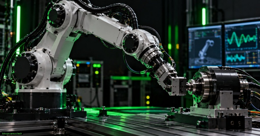
Open-Source Robotics Engineer — Lesson 005. Robot kinematics describes where a robot is and how its joints relate to end-effector motion. Trajectory planning adds desired position, velocity, and acceleration over time. Dynamics adds the missing physical question: what joint forces or torques are required to create that motion, and what motion results when forces or torques are applied?

This lesson develops the standard open-chain robot equation of motion, explains the mass matrix, Coriolis and centrifugal terms, gravity, external wrench terms, inverse dynamics, and forward dynamics, and then turns those equations into practical engineering calculations and simulation code.

Learning Objectives

• Write and interpret the manipulator equation of motion.
• Explain why the mass matrix changes with robot configuration.
• Distinguish Coriolis, centrifugal, gravity, and external-force terms.
• Use inverse dynamics to calculate required joint torque for a prescribed motion.
• Use forward dynamics to calculate joint acceleration from applied torque.
• Implement a small numerical dynamics calculation in Python.
• Recognize modeling errors involving units, inertia, friction, gravity, and coordinate conventions.

From Kinematics to Dynamics

The earlier Robotics Engineer lessons established the geometric foundation: forward kinematics and coordinate frames, Jacobians and velocity kinematics, and inverse kinematics. Those tools map joint variables into pose and velocity. Dynamics introduces mass, inertia, gravity, acceleration, and force.

For an n-joint rigid-link manipulator, a common joint-space model is:

τ = M(q) q̈ + C(q, q̇) q̇ + g(q) + J(q)ᵀ Fext + τf

Here, q is the joint-position vector, q̇ is joint velocity, q̈ is joint acceleration, τ is commanded joint force or torque, M(q) is the mass or inertia matrix, C(q,q̇)q̇ contains velocity-dependent Coriolis and centrifugal effects, g(q) is gravity compensation, J(q)ᵀFext maps an external end-effector wrench into joint space, and τf represents friction or other modeled losses.

The Mass Matrix M(q)

The mass matrix is the joint-space equivalent of mass in the familiar equation F = ma. For a multi-link robot, however, apparent inertia is not a single constant. Moving one joint accelerates several links, and changing joint configuration changes how those link masses and rotational inertias project into joint coordinates. Therefore M depends on q.

For a physically valid rigid-body model, M(q) is symmetric and positive definite away from pathological model errors. Its diagonal terms represent direct joint inertia contributions; off-diagonal terms describe inertial coupling between joints. A large off-diagonal term means acceleration at one joint can require substantial torque at another.

The robot’s kinetic energy can be written as:

T = 1/2 q̇ᵀ M(q) q̇

This relationship is useful for checking a model: with a valid positive-definite M, nonzero joint velocity produces positive kinetic energy.

Coriolis and Centrifugal Terms

The velocity-product term C(q,q̇)q̇ captures forces that appear because the robot’s coordinate system and link geometry move while the robot is already in motion. Coriolis effects couple motion between coordinates; centrifugal effects grow with rotational speed and tend to appear as squared-velocity terms. These terms disappear when q̇ = 0 but can become substantial on fast manipulators.

Engineers sometimes denote the combined velocity-dependent vector as c(q,q̇) instead of writing C(q,q̇)q̇. Both conventions are common. The important point is to keep the convention internally consistent when comparing equations, software libraries, or papers.

Gravity Compensation g(q)

Gravity torque depends on configuration. A horizontal arm generally requires more holding torque than the same arm hanging near vertical because the gravitational moment arm changes. The vector g(q) gives the joint torques required to balance gravity at a given configuration when acceleration and velocity effects are zero.

A simple one-link rotary arm illustrates the idea. For a link with mass m, center-of-mass distance l_c, joint angle q, and gravitational acceleration g, one common planar term is proportional to m g l_c cos(q), although the exact sine/cosine form depends on how the joint angle is defined. A sign error in the coordinate convention can make gravity compensation push with gravity instead of against it.

External Wrenches and the Jacobian Transpose

An end-effector force and moment can be represented by a wrench F_ext. The Jacobian transpose maps that wrench into equivalent joint torques:

τext = J(q)ᵀ Fext

This is the dynamic continuation of the force/torque duality introduced in OSREC.002. It matters in machining, force-controlled assembly, tool contact, payload handling, and any operation in which the environment pushes back on the robot.

Inverse Dynamics

Inverse dynamics asks: given q, q̇, q̈, gravity, and external load, what joint torques are required? This is the natural calculation after trajectory planning because the trajectory already specifies desired position, velocity, and acceleration as functions of time.

For an open chain, the recursive Newton–Euler algorithm computes inverse dynamics efficiently. A forward recursion propagates link positions, velocities, and accelerations from the base toward the end effector. A backward recursion propagates forces and moments from the end effector toward the base, producing the required joint forces or torques.

Forward Dynamics

Forward dynamics asks the opposite question: given q, q̇, and applied torque τ, what acceleration q̈ results? Rearranging the manipulator equation gives:

q̈ = M(q)⁻¹ [τ - C(q,q̇)q̇ - g(q) - J(q)ᵀFext - τf]

In numerical software, engineers normally avoid explicitly forming M^-1. Instead, solve the linear system M q̈ = b using a stable matrix solver. Forward dynamics is the basis of physics simulation, controller testing, digital twins, and predicting how a manipulator responds to applied torque.

Numerical Example

Assume a simplified two-joint robot at one instant has the following dynamic terms:

M = [[4.0, 1.0],
     [1.0, 2.0]] kg·m²

c = [0.5, -0.2] N·m
g = [12.0, 3.0] N·m
τ = [30.0, 10.0] N·m

Ignoring external wrench and friction, the acceleration satisfies Mq̈ = τ – c – g. The right-hand side is [17.5, 7.2] N·m. Solving the 2×2 system gives approximately q̈ = [3.97, 1.62] rad/s². Notice that the off-diagonal inertia terms couple the joints; the accelerations are not simply torque divided by each diagonal element.

Python Example: Solve Forward Dynamics

import numpy as np

M = np.array([[4.0, 1.0],
              [1.0, 2.0]])

c = np.array([0.5, -0.2])
g = np.array([12.0, 3.0])
tau = np.array([30.0, 10.0])

rhs = tau - c - g
qdd = np.linalg.solve(M, rhs)

print("joint acceleration rad/s^2:", qdd)

For production robotics software, M, c, and g are computed from the robot model at the current state rather than typed by hand. Libraries may use URDF inertial parameters, spatial-vector algebra, recursive Newton–Euler methods, articulated-body algorithms, or automatically generated rigid-body dynamics code.

Model Parameters Must Be Physically Correct

A dynamics model is only as good as its mass properties. Each link needs realistic mass, center-of-mass location, and inertia tensor. Motors, gearboxes, tooling, cables, payloads, and fixtures may also contribute meaningful reflected inertia or friction. A robot that looks geometrically correct in simulation can still have completely wrong torque predictions if its inertial parameters are placeholders.

Check units carefully: kilograms for mass, meters for dimensions, kg·m² for rotational inertia, newtons for force, newton-meters for torque, radians for angular position, radians per second for angular velocity, and radians per second squared for angular acceleration. Millimeters accidentally interpreted as meters can corrupt inertia by orders of magnitude.

Dynamics and Simulation

A simulator repeatedly evaluates forward dynamics and numerically integrates acceleration to update velocity and position. A simple conceptual loop is:

while simulation_running:
    M = mass_matrix(q)
    bias = coriolis_and_centrifugal(q, qd) + gravity(q)
    qdd = solve(M, tau - bias)

    qd = qd + qdd * dt
    q = q + qd * dt

This simple Euler integration is useful for understanding the signal flow but may be inaccurate or unstable for stiff systems or large time steps. Production simulators often use smaller time steps, higher-order integration, constraint solvers, contact models, and actuator models.

Engineering Checks and Troubleshooting

• Static gravity check: set q̇ = 0 and q̈ = 0. Required torque should reduce mainly to gravity plus external load and static friction.
• Zero-gravity check: disable gravity in simulation. A stationary robot with zero applied torque should not spontaneously accelerate because of a gravity term.
• Energy check: in an ideal frictionless, unforced simulation, total mechanical energy should remain approximately constant; significant drift can indicate integration or model problems.
• Symmetry check: M should be numerically symmetric within tolerance.
• Positive-definite check: physically valid inertia should not produce negative kinetic energy.
• Sign check: verify gravity direction, joint-axis direction, and wrench conventions.
• Payload check: repeat torque calculations with and without the tool payload and compare the difference.

Exercises

1. For a one-joint rotary link, explain why holding torque changes as the arm moves from vertical to horizontal.
2. Using the numerical two-joint example above, change τ to [20, 5] N·m and solve for q̈.
3. Modify the Python example to add an external-joint torque vector τext = [2, -1] N·m and subtract it from available actuator torque.
4. Write a diagnostic procedure for a simulated robot that falls upward when gravity is enabled.
5. Explain why directly computing np.linalg.inv(M) @ rhs is usually less desirable than np.linalg.solve(M, rhs).

Knowledge Check

1. What does M(q) represent?
2. Why does the mass matrix depend on robot configuration?
3. When do Coriolis and centrifugal terms vanish?
4. What does inverse dynamics calculate?
5. What does forward dynamics calculate?
6. How is an end-effector wrench mapped into joint torques?
7. What should a static gravity-compensation test set q̇ and q̈ to?
8. Why can an accurate geometric model still produce inaccurate torque predictions?

Knowledge Check Answers

1. M(q) is the configuration-dependent joint-space mass/inertia matrix.
2. Changing configuration changes how each link’s mass and rotational inertia project into joint motion and how joints are inertially coupled.
3. They vanish when joint velocity q̇ is zero.
4. Inverse dynamics calculates the joint forces or torques required to produce a specified q, q̇, and q̈ under modeled loads.
5. Forward dynamics calculates q̈ from the current state and applied joint forces or torques.
6. Through the Jacobian transpose: τext = J(q)ᵀFext.
7. Set both q̇ and q̈ to zero.
8. Because dynamics also requires accurate masses, centers of mass, inertia tensors, payload properties, friction, gravity, and actuator parameters.

Continue the Robotics Engineer Track

Review OSREC.001 for kinematics and frames, OSREC.002 for Jacobians and statics, OSREC.003 for numerical inverse kinematics, and OSREC.004 for trajectory generation. Together, those lessons provide the geometric and motion-planning inputs needed for the dynamic calculations developed here.

BitcoinVersus.Tech

Editor’s Note

This lesson follows standard rigid-body robotics notation. Textbooks and software libraries may group Coriolis and centrifugal effects differently or use alternate signs for external wrench terms; always verify the convention used by the specific model or library.

Support and donation options are available through BitcoinVersus.Tech.

BitcoinVersus.tech is not a financial advisor. Content is provided for informational purposes.