Learning Objectives

• Interpret the rigid-manipulator equation τ = M(q)q̈ + C(q,q̇)q̇ + g(q) + τf.
• Explain how configuration, payload, gravity, velocity, and acceleration change joint effort.
• Distinguish forward dynamics from inverse dynamics.
• Calculate torque for a single rotational joint and implement the model in Python.
• Describe computed-torque control and identify practical limits of model-based control.

Required Foundation

• OSREC.001: Robot Kinematics and Coordinate Frames
• OSREC.002: Robot Jacobians
• OSREC.003: Inverse Kinematics
• OSREC.004: Robot Trajectory Planning

Dynamics From Motion To Torque

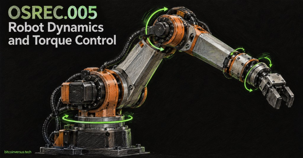
Robot kinematics determines where a mechanism can move; dynamics determines the force or torque required to produce that motion. For independent joint coordinates q, a standard rigid-link model is τ = M(q)q̈ + C(q,q̇)q̇ + g(q) + τf. The vector τ contains actuator effort, M(q) is the configuration-dependent mass matrix, C(q,q̇)q̇ contains velocity-dependent Coriolis and centrifugal effects, g(q) is gravity loading, and τf represents friction. Revolute-joint effort is measured in newton-metres; prismatic-joint effort is measured in newtons.

Mass Matrix, Gravity, And Payload

The mass matrix is not a fixed collection of motor inertias: it normally changes with joint configuration and includes off-diagonal coupling terms. A simple point mass m located a distance r from a rotational axis contributes I = mr² to rotational inertia. Moving the same mass farther from the axis therefore increases acceleration torque quadratically, while its gravity moment grows with the lever arm. A valid model must include the mounted tool and payload, calibrated joint encoders, the relevant actuator limits, and the losses and ratios of the drive system.

Forward And Inverse Dynamics

Inverse dynamics starts with q, q̇, and q̈ and computes the effort τ required to follow the commanded motion. Forward dynamics starts with the current state and applied effort and solves q̈ = M(q)⁻¹[τ − C(q,q̇)q̇ − g(q) − τf]. Numerical software should solve the linear system rather than explicitly form M⁻¹. The recursive Newton–Euler algorithm evaluates inverse dynamics efficiently along a serial chain, making it suitable for trajectory analysis and real-time control.

Worked Single-Joint Example

Consider a horizontal rotary link with effective inertia I = 0.24 kg·m², angular acceleration q̈ = 3.0 rad/s², viscous coefficient b = 0.08 N·m·s/rad, angular velocity q̇ = 1.5 rad/s, payload mass m = 2.0 kg, centre-of-mass radius r = 0.30 m, and angle q = 30° measured from the horizontal. Using τ = Iq̈ + bq̇ + mgr cos(q), the inertia term is 0.72 N·m, friction is 0.12 N·m, gravity is approximately 5.10 N·m, and total required torque is approximately 5.94 N·m. The result demonstrates why slowing a trajectory reduces acceleration effort but does not remove static gravity demand.

from math import cos, radians

I = 0.24      # kg·m²
q_ddot = 3.0  # rad/s²
b = 0.08      # N·m·s/rad
q_dot = 1.5   # rad/s
m = 2.0       # kg
r = 0.30      # m
g = 9.81      # m/s²
q = radians(30)

tau_inertia = I * q_ddot
tau_friction = b * q_dot
tau_gravity = m * g * r * cos(q)
tau_total = tau_inertia + tau_friction + tau_gravity

print(f"Required torque: {tau_total:.2f} N·m")

Computed-Torque Control

Computed-torque control uses the dynamics model to cancel predicted nonlinear behavior and impose a simpler tracking-error response. With desired position qd, desired velocity q̇d, and desired acceleration q̈d, define e = qd − q and command τ = M(q)[q̈d + Kdė + Kpe] + C(q,q̇)q̇ + g(q). Perfect cancellation is only theoretical: uncertain payloads, friction, backlash, elasticity, sensor noise, delay, saturation, and contact forces create model error. Gain selection must preserve stability and remain inside continuous torque, peak torque, speed, thermal, and braking limits.

Practical Exercises

1. Recalculate the worked example with the payload radius increased from 0.30 m to 0.45 m. Compare the gravity torque and point-mass inertia contribution.
2. Set q̈ = 0 and q̇ = 0. Calculate the holding torque at q = 0°, 45°, and 90°.
3. Modify the Python example to evaluate angles from 0° through 180° in 15° increments and report the maximum absolute torque.
4. For a two-joint model, explain why an off-diagonal mass-matrix term can make joint 1 torque change when only joint 2 acceleration changes.
5. Create a validation checklist covering payload data, encoder zero, friction, torque saturation, emergency braking, and temperature limits.

Knowledge Check

1. Which dynamics term maps joint acceleration to inertial effort?
2. What is the primary difference between forward and inverse dynamics?
3. Why can a slower motion still exceed an actuator’s continuous torque rating?
4. Why should numerical software solve a linear system instead of explicitly calculating M⁻¹?
5. Name four effects that can make computed-torque cancellation imperfect.

Answer Key

1. The mass matrix M(q).
2. Forward dynamics computes acceleration from state and applied effort; inverse dynamics computes required effort from state and desired acceleration.
3. Static gravity torque and repeated thermal loading remain even when acceleration is reduced.
4. A direct linear solve is generally more accurate and efficient than constructing an explicit inverse.
5. Examples include payload uncertainty, friction, backlash, compliance, sensor noise, delay, saturation, and unmodeled contact forces.

BitcoinVersus.Tech

Editor’s Note

This certificate lesson is an educational treatment of robot dynamics. Equations and software examples use idealized models and are not commissioning instructions for physical machinery.

Support And Donation

Support independent technical education through the donation options published on BitcoinVersus.Tech.

Disclaimer

Educational content only. Verify calculations, safety limits, manufacturer documentation, applicable standards, and site procedures before operating or modifying equipment.