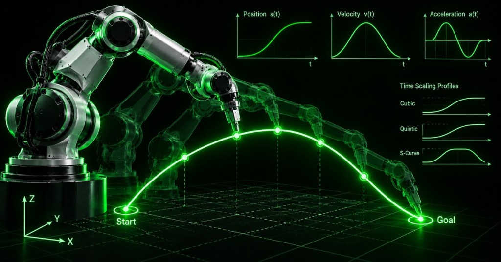
A robot trajectory is more than a destination. It specifies how an industrial robot should move from one configuration to another as time advances, including the path, speed, acceleration, and smoothness of the motion. OSREC.004 continues from OSREC.001 kinematics, OSREC.002 Jacobians, and OSREC.003 inverse kinematics by adding the missing time dimension.

Path Versus Trajectory

A path describes where the robot goes; a trajectory describes where it goes and when it is at each point. A path can be written as q(s), where the path parameter s moves from 0 to 1, while time scaling supplies s(t). The executed trajectory is therefore q(t) = q(s(t)). By the chain rule, q̇ = (dq/ds)ṡ and q̈ = (d²q/ds²)ṡ² + (dq/ds)s̈. This separation is important because the same geometric path can be executed slowly, quickly, or with different acceleration profiles without changing its shape.

Joint-Space and Cartesian Paths Solve Different Problems

In joint-space planning, each joint angle moves between start and goal values, often making joint limits straightforward to check, but the tool may trace a curved route through the workspace. In Cartesian planning, the tool or Tool Center Point follows a desired line or pose path in physical space, so inverse kinematics must continuously map that path back into joint coordinates. Cartesian motion is useful for welding, dispensing, insertion, machining, and other processes where the end-effector route matters; joint-space motion is often simpler when only the final pose matters.

Cubic, Quintic, Trapezoidal, and S-Curve Profiles

For normalized time τ = t/T, a common cubic scaling is s(τ)=3τ²−2τ³; it starts and ends with zero velocity, but its acceleration jumps at the endpoints. A quintic scaling, s(τ)=10τ³−15τ⁴+6τ⁵, also forces endpoint acceleration to zero. Trapezoidal velocity profiles use constant acceleration, constant velocity, and constant deceleration. S-curves go one step further by shaping jerk, the derivative of acceleration, which reduces abrupt changes in force and can improve motion quality in the robot drive system. Smoothness therefore has a hierarchy: position → velocity → acceleration → jerk.

Via Points Shape the Route Without Requiring Stops

A practical robot rarely moves only from one isolated start pose to one isolated goal. Engineers often define via points or waypoints that shape the route around fixtures, align the tool before contact, or enforce process geometry. Polynomial interpolation can connect these points while maintaining continuity in position and velocity. The engineering requirement is not merely to “hit every point,” but to make adjacent segments agree on enough derivatives that the robot does not command an impossible instantaneous change in velocity or acceleration. Via-point timing also matters: squeezing the same geometric path into less time raises required velocity and acceleration.

Dynamic Limits Turn Geometry Into an Engineering Constraint

A geometrically valid trajectory may still be dynamically impossible. Joint velocity limits, acceleration limits, motor torque, gearbox loading, payload, gravity, friction, and thermal constraints bound how quickly the robot can follow a path. If ṡ becomes too large, available actuator torque may no longer provide an allowable s̈ that keeps the robot on the commanded path. Time-optimal planning therefore seeks the fastest valid time scaling that remains inside the robot’s dynamic limits, but maximum-throughput motion is not automatically the best production motion because model error, wear, vibration, payload uncertainty, and safety margin still matter.

Planning Software Separates Path Search From Trajectory Execution

Modern robotics software typically separates several layers: a planner searches for a feasible path, a trajectory generator or time-parameterization stage assigns velocities and accelerations, and a lower-level controller sends commands to the actuators. MoveIt, maintained in the ecosystem around PickNik, is a common open-source framework for manipulator motion planning, while ROS supplies the broader communication and control environment. This layered architecture is useful for debugging because a bad path, bad time parameterization, and bad controller tracking produce different failure signatures.

Execution Must Be Verified Against the Real Robot

The commanded trajectory is only a reference; the physical robot follows it using feedback from encoders and the controller. Engineers should compare commanded and measured position, velocity, and following error; inspect whether velocity or torque limits are clipping the motion; and confirm that the actual TCP stays on the intended path. If the plan is smooth but tracking oscillates, the control loop or mechanical system may be the problem. If the controller tracks perfectly but the end effector takes the wrong geometric route, the path or kinematic model is the better suspect.

Worked Example: 90° Joint Move in 3 Seconds

• Initial joint angle: q₀ = 0°
• Final joint angle: qf = 90°
• Total time: T = 3 s
• Cubic scaling: s(τ)=3τ²−2τ³, where τ=t/T
• Trajectory: q(t)=q₀+(qf−q₀)s(t)
• At t=1.5 s: τ=0.5, s=0.5, so q=45°
• Peak cubic velocity: 45°/s at the midpoint
• Endpoint acceleration magnitude: 60°/s², showing why cubic scaling has a nonzero acceleration step at the endpoints

Minimal Quintic Generator

tau = t / T
s = 10*tau**3 - 15*tau**4 + 6*tau**5
q = q0 + (qf - q0) * s

Trajectory Engineering Checklist

1. Define the start and goal configurations or poses.
2. Choose joint-space, Cartesian, screw, or another appropriate path representation.
3. Check reachability, joint limits, singularities, and collision constraints.
4. Add via points only when they express a real process or clearance requirement.
5. Choose a time-scaling profile appropriate for the required smoothness.
6. Verify joint velocity, acceleration, jerk, torque, and payload limits.
7. Time-parameterize the path without violating actuator limits.
8. Simulate the trajectory before physical execution.
9. Run the real robot at reduced speed first.
10. Compare commanded and measured joint states and TCP motion.
11. Record following error, saturation, vibration, and cycle time.
12. Retain safety and reliability margin rather than automatically selecting the mathematical minimum time.

Exercises

1. Explain the difference between a path q(s) and a trajectory q(s(t)).
2. For the cubic time scaling, differentiate s(τ)=3τ²−2τ³ to obtain normalized velocity and acceleration.
3. Compare the endpoint conditions satisfied by cubic and quintic time scaling.
4. Explain why a straight line in joint space does not generally produce a straight-line TCP path.
5. Design three via points for a robot that must approach a fixture from above.
6. Explain why halving move time can sharply increase required acceleration and torque.
7. Describe one application where S-curve motion is preferable to a trapezoidal velocity profile.
8. Separate a motion-planning failure from a trajectory-tracking failure using observable evidence.
9. Explain why time-optimal motion may be undesirable on a real production robot.
10. Propose acceptance limits for position error, velocity error, and cycle time during trajectory validation.

Knowledge Check + Answers

1. What does time scaling do? It maps time into progress along a geometric path, determining how quickly the path is followed.
2. What is jerk? The time derivative of acceleration.
3. Why use quintic instead of cubic scaling? Quintic scaling can enforce zero velocity and zero acceleration at both endpoints.
4. What is a via point? An intermediate configuration or pose used to shape a trajectory.
5. Why can a valid path still be impossible to execute? Joint velocity, acceleration, torque, collision, singularity, or other dynamic constraints may be violated.
6. What does a velocity-limit curve represent in time-optimal scaling? The maximum feasible path speed at each location under the robot’s dynamic constraints.
7. What is the difference between planning and control? Planning generates a desired path/trajectory; control drives the physical robot to track that reference.
8. Why compare commanded and measured trajectories? The difference exposes tracking errors, saturation, mechanical issues, model mismatch, and controller problems.

Reference Resources

• Northwestern University — Modern Robotics, Chapter 9: Trajectory Generation
• MoveIt — Trajectory Processing documentation

Key Takeaway

Inverse kinematics tells a robot which joint configuration can reach a target; trajectory planning tells the robot how to move there over time. Good trajectory engineering separates geometry from timing, chooses the right joint-space or Cartesian representation, controls velocity, acceleration, and jerk, respects actuator and payload limits, and verifies the commanded motion against measured encoder feedback. That is the bridge between a mathematically reachable pose and motion that a real robot can execute smoothly, safely, and repeatably.

BitcoinVersus.Tech

Advertisement

Use the #promocode bitcoinversus at check out to Get 5% off #Bitaxe Mining Products

Limited to one use per customer Happy #Bitcoin Mining!https://t.co/0trBgXkbVd

— BitcoinVersus.Tech 📟 (@1BitcoinVersus) June 23, 2025

Editor’s Note:

We volunteer daily to ensure the credibility of the information on this platform is Verifiably True. If you would like to support our research initiatives, please donate here: 3C9o19EH5HSiwEPyCTmEKzxhNCbo2X6TTb

BitcoinVersus.tech is not a financial advisor. This media platform reports on financial subjects purely for informational purposes.