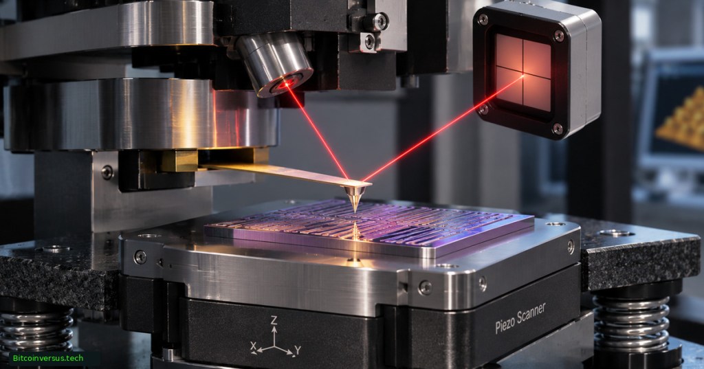
An atomic force microscope (AFM) measures a material’s surface by moving a sharp probe across it and recording interactions between the tip and the sample. Its calibrated output is a height map, often capable of subnanometer vertical detail. For semiconductor manufacturers, AFM can quantify wafer roughness, patterned-feature height, line width and local material behavior. However, the result is ordinarily a surface map, sometimes called 2.5D topography, not a complete volumetric picture of everything beneath a chip’s surface.

AFM was introduced by Gerd Binnig, Calvin Quate and Christoph Gerber in a March 3, 1986 paper. Their early demonstration reported 30 ångströms (3 nm) lateral resolution and less than 1 ångström (0.1 nm) vertical resolution. The figures described an early experiment, not the guaranteed accuracy of every modern instrument. Forty years later, NIST uses AFM to develop traceable nanometer-scale measurement standards.

How an AFM actually measures a surface

A flexible cantilever carries a tip toward the sample. In many instruments, a laser reflects from the cantilever onto a position-sensitive photodetector. Changes in the measured signal feed a control loop that adjusts the probe or specimen’s vertical position while a scanner moves in X and Y. The recorded Z signal constructs a height map. Other AFMs use electrical self-sensing probes rather than laser deflection. Nanosurf’s engineering reference describes scanner, calibration and feedback arrangements.

Common operating modes include contact, intermittent contact or tapping, and noncontact. Contact mode maintains tip contact but can impose lateral forces on sensitive materials. Tapping reduces continuous sliding contact. Noncontact operation avoids intentional touching, yet its signal depends on force gradients, atmosphere and feedback. No mode is universally free of sample damage or artifacts. The semiconductor inspection primer places AFM alongside optical inspection and electron-beam techniques.

The scan-density equation

An AFM height image records approximately N × N samples for a square N-pixel raster. A 128 × 128 scan contains 16,384 height samples; 256 × 256 has 65,536; and 512 × 512 has 262,144. Doubling pixels per axis therefore quadruples image samples. Moving from 128 to 512 creates 16 times the data points, not necessarily 16 times more physical detail. The example settings appear in Purdue University’s 2025 AFM training guide.

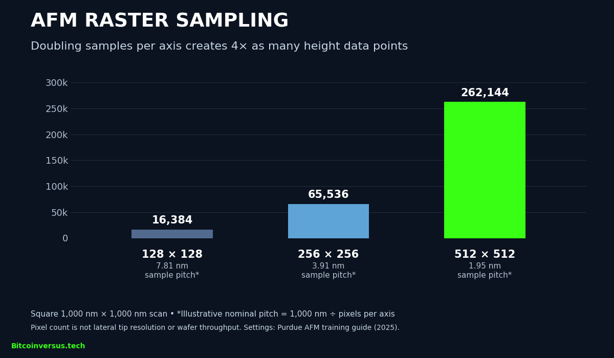
For a 1,000-nm-wide scan, nominal sample spacing is width divided by pixels per line: approximately 7.81 nm at 128 pixels and 1.95 nm at 512. Tip radius, probe wear, calibration, drift and feedback can limit feature resolution even when the pixel grid is dense. A surface-roughness reference explains why roughness statistics must be interpreted with the scan area and preparation method.

NIST’s subnanometer calibration example

In an August 19, 2026 publication, NIST researcher Gheorghe Stan described a multipoint AFM height-calibration method using steps on a silicon-carbide surface. The reported calibration steps ranged from 0.756 nm to heights approaching 50 nm, spanning roughly a 66-fold height scale. The range characterizes reference features used to test Z-axis linearity; it is not a claim of 0.756-nm instrument accuracy or a 66-fold productivity gain.

Why chip fabs use AFM alongside SEM and optics

AFM excels at local surface-height measurements and can also probe adhesion, stiffness, electrical potential and nanoscale mechanical response through specialized modes. An NIST 2026 hybrid-bonding study used three AFM modes to characterize copper and silica patterns relevant to chip stacking. Optical tools remain valuable for faster large-area inspection, and scanning electron microscopes provide different kinds of feature contrast and imaging. See BitcoinVersus.Tech’s electron- and ion-beam comparison. No single tool replaces the others.

AFM also faces tip-convolution errors when a finite-width tip encounters a narrow structure, inaccessible undercuts, vibration, thermal drift and limited scan speed. NIST emphasizes calibrated tips, traceability and uncertainty budgets. Surface height data alone cannot establish chemical composition, buried-device integrity or semiconductor yield; the wafer-yield engineering guide distinguishes measurements from good-die statistics.

Industrial innovation now targets parallel sampling. A separate November 2026 report on eight-head AFM examines an emerging prototype. More heads do not automatically mean proportional wafer throughput; independent fab qualification must establish repeatability, accuracy, scan time and contamination controls.

Primary references: Binnig, Quate and Gerber (1986); NIST AFM program; Stan’s 2026 calibration study; NIST mechanical/electrical AFM program; Nanosurf operating principles.

Editor’s Note: An AFM height map has quantitative Z information but is generally not a volumetric reconstruction. The 1986 sub-ångström vertical result is historical, and the 2026 NIST value of 0.756 nm identifies a calibration step, not certified instrument accuracy. The raster chart presents arithmetic based on stated training settings rather than measured device throughput. The featured cover is a conceptual illustration; manufacturer videos depict general AFM principles. Full video playback and independent cross-device appearance checks have not been confirmed.

Support BitcoinVersus.Tech

To support independently researched educational reporting, scan the original approved QR code below for an optional 5,000-satoshi donation. Mobile readers can open the page on a second display or use the wallet’s scan-from-image feature when available. Verify the receiving address and amount before paying.

We volunteer daily to ensure the information on this platform is Verifiably True. If you would like to support the research, please scan QR code.