Elementary Overview

A robot trajectory planner can generate an ideal motion, but the real machine still needs a feedback controller to follow that motion while dealing with gravity, friction, payload changes, sensor noise, model error, and external disturbances. This lesson builds on OSREC.004: Robot Trajectory Planning and OSREC.005: Robot Dynamics. The planner says where the robot should go; the controller decides how to continuously correct the difference between the desired motion and the measured motion.

The core idea is a closed loop: desired state → controller → actuator command → robot → sensor measurement → error → controller again. The robot’s servo drives and encoders make that loop physically possible. Without feedback, the system is open-loop and cannot directly correct for what actually happened.

Control Starts With Error

For one robot joint, define the position error as e = θ_d − θ, where θ_d is the desired joint position and θ is the measured joint position. If the joint is behind the commanded trajectory, the error is positive. If it has moved past the desired position, the error changes sign. The controller uses that error, and sometimes its history and rate of change, to calculate the next command.

In a multi-joint robot, the same idea becomes a vector relationship. The desired joint configuration comes from the trajectory generator, while the actual configuration comes from joint encoders. The controller continuously drives the error vector toward zero while respecting actuator, velocity, acceleration, and safety limits.

Proportional Control Reacts To Present Error

The simplest feedback term is proportional control. A proportional controller produces a command that grows with the current error: larger error creates a stronger correction, while smaller error creates a weaker correction. In compact form, the control contribution is K_pe.

Increasing K_p usually makes the response faster, but excessively high gain can produce oscillation, vibration, actuator saturation, or instability once real delays, flexible mechanics, sampling, noise, and unmodeled dynamics are included. This is why “turn the gain up until it is fast” is not a sound tuning method for a real robot.

Integral Control Accumulates Persistent Error

A proportional controller may leave a steady tracking offset when a constant command is required to overcome gravity, friction, or a continuously moving trajectory. Integral control addresses this by accumulating error over time. Its contribution is proportional to the time integral of e, written conceptually as K_i∫e dt.

If a small error remains for many control cycles, the integral term keeps growing until it produces enough command to remove that persistent offset. This can be extremely useful, but the integral state must be managed carefully. If an actuator saturates while the integrator keeps accumulating error, the controller can suffer integral windup, leading to overshoot or slow recovery after the saturation ends.

https://www.youtube.com/watch?v=NAXmXg1gCI0

Derivative Control Adds Damping

Derivative control responds to how quickly the error is changing. In a joint-position controller, the derivative contribution is commonly related to joint velocity error and acts like a virtual damper. Its conceptual form is K_dė. If the robot is approaching the target too quickly, derivative action can reduce the command before the joint overshoots.

This is especially important in mechanical systems because position correction alone can create a spring-like response. Adding derivative action introduces damping and can turn an oscillatory response into a critically damped or near-critically damped one. The tradeoff is that differentiation amplifies measurement noise, so practical systems often filter the velocity or derivative signal rather than differentiating raw noisy position measurements directly.

PID Combines Present, Past, And Rate Of Change

A PID controller combines proportional, integral, and derivative action. The conceptual torque command is τ = K_pe + K_i∫e dt + K_dė. The proportional term reacts to present error, the integral term removes persistent offset, and the derivative term adds damping based on motion.

Many robot joint controllers use PD or PID-like structures internally even when the user never sees the raw gains. Industrial controllers often layer these loops: fast motor-current control inside velocity control, with position control outside both. The exact architecture is manufacturer-specific, but the general control hierarchy explains why a modern industrial robot can regulate motor torque, joint velocity, and joint position at different bandwidths.

https://www.youtube.com/watch?v=HAVBtupm8zM

Feedforward Uses The Desired Motion Before Error Appears

Feedback waits for error to exist before correcting it. Feedforward improves tracking by using known desired motion to command part of the required action in advance. For a velocity-controlled robot, the desired joint velocity can be added directly to the feedback command. For a torque-controlled robot, a dynamic model can estimate how much torque is required for desired acceleration, gravity compensation, and other predictable effects.

The strongest practical controller is therefore often not “feedback versus feedforward.” It is feedforward plus feedback. Feedforward handles what the model already predicts, while feedback corrects model mismatch, disturbances, friction uncertainty, payload variation, and measurement error.

Trajectory Tracking Is Different From Holding A Setpoint

A robot holding one fixed joint angle is performing setpoint control. A robot following θ_d(t) through time is performing trajectory tracking. The second problem is harder because the target itself is moving. The controller must reduce position error while also matching desired velocity and, in higher-performance systems, desired acceleration.

This is why the output of trajectory planning typically contains position, velocity, and acceleration references rather than only a final point. A smooth trajectory gives the controller physically reasonable commands; a discontinuous or overly aggressive trajectory can demand impossible accelerations and force the servo system into saturation.

Joint-Space And Task-Space Control Solve Different Problems

In joint-space control, each joint tracks a desired angle trajectory. This is conceptually simple and maps naturally to motor encoders and joint servo loops. In task-space control, the desired error is defined at the end effector in Cartesian position and orientation.

Task-space control depends on the robot Jacobian to connect end-effector motion to joint motion. Near a kinematic singularity, small desired task-space motion can require very large joint velocities, so the control law must account for conditioning, limits, and the geometry of the manipulator.

Robot Dynamics Change How Gains Feel

The same controller gains do not necessarily produce the same response everywhere in the robot workspace. The effective inertia seen by a joint changes with configuration, payload, and the coupling between links. Gravity torque changes as the arm moves. Friction and cable forces also vary.

This is the direct connection to robot dynamics. A simple PID controller treats those effects as disturbances to be corrected after error appears. A model-based controller can instead use the mass matrix, Coriolis/centrifugal terms, and gravity model to cancel or compensate much of the predictable dynamics before the feedback terms clean up the remaining error.

https://www.youtube.com/watch?v=MV-xBPP3H2k

Gain Tuning Is A Tradeoff, Not A Maximum-Number Contest

Increasing K_p usually increases stiffness and reduces position error, but too much proportional gain can excite structural flexibility, gearbox compliance, backlash, or sampling delay. Increasing K_d adds damping, but too much derivative action can amplify noise and create excessive control effort. Increasing K_i removes steady-state error, but too much integral action can create overshoot and windup.

Good tuning therefore balances settling time, overshoot, steady-state error, noise sensitivity, actuator effort, and robustness. A critically damped or slightly underdamped response is often a useful engineering target, but real industrial controllers may also use notch filters, friction compensation, gain scheduling, adaptive terms, current limits, velocity limits, and proprietary servo algorithms.

Actuator Saturation Changes The Controller

Every real robot has finite motor torque, current, velocity, and acceleration. If the controller requests more than the actuator can deliver, the command saturates. Once saturation occurs, the mathematical controller is no longer behaving like the ideal unsaturated model used in analysis.

This matters most for integral control because the integrator can continue accumulating error even when the actuator is pinned at its limit. Anti-windup strategies pause, clamp, or back-calculate the integral state so the controller can recover more cleanly when the actuator returns to its controllable range.

Sampling Rate And Delay Affect Stability

Robot control software runs in discrete time. Encoders are sampled, calculations take time, networked signals have delay, and the drive updates its command on a schedule. A controller that is stable in a continuous-time equation can become unstable if implemented with too much delay or with gains that are too aggressive for the sampling rate.

Fast inner servo loops are one reason industrial robot drives are tightly integrated with the controller. Position, velocity, and current loops operate at different rates so that the fastest electrical dynamics are handled closest to the motor while slower planning and application logic operate farther outside the loop.

Control Errors Can Look Like Mechanical Faults

Poor gain tuning can produce oscillation, overshoot, buzzing, slow settling, or tracking error that looks like loose mechanics. The reverse is also true: backlash, loose couplings, encoder problems, incorrect payload data, damaged reducers, or friction can make a correctly designed controller appear poorly tuned.

That is why a control engineer must separate software behavior from hardware condition. If a robot suddenly begins oscillating after maintenance, inspect alarm history, encoder integrity, mechanical coupling, payload, and servo condition before changing gains. Tuning should not be used to hide a broken mechanism.

Worked Example: One Joint Tracking A Ramp

• Desired motion: the joint angle increases at constant velocity.
• P only: the joint follows the motion but can remain a fixed distance behind because nonzero error is required to produce a nonzero corrective command.
• PI: the integral term accumulates the persistent offset and can drive steady-state tracking error toward zero.
• Feedforward + PI: the desired velocity is commanded directly while PI feedback corrects disturbances and modeling error.
• Engineering lesson: use feedforward for what is known in advance and feedback for what reality changes.

Engineering Checklist

1. Define the controlled variable: joint position, velocity, torque, or task-space pose.
2. Define the desired trajectory and its position, velocity, and acceleration references.
3. Verify encoder and sensor signals before tuning.
4. Start with stable conservative gains rather than maximum gains.
5. Increase proportional action until response is sufficiently stiff without sustained oscillation.
6. Add derivative damping where needed and monitor noise sensitivity.
7. Add integral action only when persistent error justifies it.
8. Implement anti-windup when actuator saturation is possible.
9. Use feedforward for known desired velocity, acceleration, gravity, or model-based torque where appropriate.
10. Check torque, current, velocity, and acceleration limits during tuning.
11. Test across representative payloads and robot configurations.
12. Verify tracking in both joint space and task space when the application depends on end-effector accuracy.

Exercises

1. Explain the difference between open-loop and closed-loop robot control.
2. Describe what happens when K_p is too low and when it is too high.
3. Explain why integral action can remove steady-state error.
4. Explain how derivative action adds damping.
5. Describe integral windup and one anti-windup strategy.
6. Explain why feedforward can reduce tracking error before feedback acts.
7. Describe why one set of gains may behave differently at different robot configurations.
8. Explain why a trajectory with unrealistic acceleration demands can force the controller into saturation.

Knowledge Check + Answers

1. What does proportional control use? The current error between desired and measured state.
2. What does integral control use? The accumulated error over time.
3. What does derivative control use? The rate of change of error, commonly related to velocity error.
4. Why combine feedforward and feedback? Feedforward handles predictable desired motion while feedback corrects disturbances and model error.
5. What is integral windup? Excessive buildup of integral state while an actuator is saturated or unable to follow the requested command.
6. Why can high gains destabilize a real robot? Delay, sampling, actuator limits, flexible mechanics, sensor noise, and unmodeled dynamics violate ideal assumptions.
7. How does the Jacobian enter task-space control? It maps between joint motion and end-effector motion so Cartesian error can be converted into joint-level commands.

Prior Lessons And References

• OSREC.001 — Robot Kinematics and Coordinate Frames
• OSREC.002 — Robot Jacobians
• OSREC.003 — Inverse Kinematics
• OSREC.004 — Robot Trajectory Planning
• OSREC.005 — Robot Dynamics
• Modern Robotics — Motion Control With Velocity Inputs
• Modern Robotics — PID/PD Motion Control With Torque Inputs
• Modern Robotics — Feedforward, Feedback, and Model-Based Torque Control
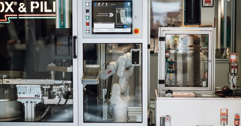
• Featured source photo — Shixart1985/Nenad Stojkovic via Wikimedia Commons, CC BY 2.0; cropped to 1200×630.

Elementary Conclusion

Robot feedback control closes the gap between an ideal trajectory and a physical machine. Proportional action corrects present error, integral action removes persistent offset, derivative action adds damping, and feedforward uses known desired motion before error develops. Good control engineering is not simply choosing large gains: it is balancing tracking accuracy, stability, noise, actuator limits, sampling, dynamics, and mechanical reality. Once these ideas are understood, trajectory planning and robot dynamics become a complete motion system rather than isolated equations.

BitcoinVersus.Tech

Advertisement

BitcoinVersus.Tech publishes open technical education across robotics, control systems, electronics, programming, semiconductors, networking, and data centers.

Editor’s Note

Controller gains, loop rates, torque limits, filtering, safety limits, and tuning procedures are robot- and drive-specific. Follow the manufacturer’s documentation and approved test procedure before modifying production servo parameters.

We volunteer daily to help keep the information on this platform verifiably accurate. Support our independent research through the support options available on BitcoinVersus.Tech.

BitcoinVersus.tech is not a financial advisor. Content is provided for informational purposes.