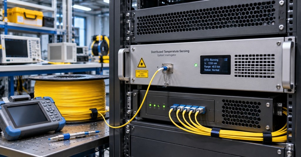
OSFOEC.014 explains how fiber-optic cables become distributed temperature sensors across kilometers of an industrial route. A distributed temperature sensing (DTS) interrogator launches light into glass and analyzes backscattered photons whose spectral properties contain temperature information. Engineers must transform the signals into calibrated measurements, connect optical distance to actual infrastructure coordinates, and verify the meaning of alarms before declaring a physical hotspot.

The chapter advances beyond OSFOEC.013 on bidirectional OTDR. Ordinary telecom OTDR measures reflections and attenuation; Raman-DTS infers temperature using different parts of the scattered spectrum. Previous chapters on reflectance and return loss, optical scattering and nonlinear effects and OTDR field testing provide the scientific and measurement prerequisites.

Learning objectives and prerequisites

• Describe Raman Stokes and anti-Stokes scattering, their optical energy shifts, and their relation to temperature.
• Distinguish Raman-DTS, Brillouin temperature-and-strain sensing and Rayleigh distributed acoustic sensing.
• Calculate the approximate round-trip optical delay for a known fiber length.
• Separate sample spacing, spatial resolution, location accuracy, temperature accuracy, and integration time.
• Explain why reference-temperature calibration, differential attenuation and surveyed route locations matter.
• Interpret simulated temperature profiles without mistaking them for physical test results.
• Produce an evidence-based engineering report with fault hypotheses, uncertainty and safe escalation requirements.

The necessary background includes single-mode fiber propagation, optical attenuation, OTDR event tables and basic statistics. For a documentation-only lesson, a calculator, spreadsheet or standard Python 3 environment is sufficient. Do not connect or disconnect optical fibers or manipulate installed power cable monitoring without approved procedures and qualified supervision.

Fiber as a distributed temperature instrument

Unlike a discrete thermometer installed at one enclosure, a suitable sensing fiber can report temperatures at many positions along its cable route. The U.S. Environmental Protection Agency’s open fiber-optic DTS tutorial describes pulsed measurement, calibrated temperature and the difference between optical and mapped physical distances. Real applications range from environmental research to monitoring buried electrical cables and pipelines.

DTS technologies are not interchangeable. Raman systems primarily derive temperature from Stokes and anti-Stokes intensity relationships. Brillouin frequency shifts respond to strain as well as temperature; separating those contributions may require an additional reference or experimental model. Rayleigh-based techniques can be used for acoustic or other sensing modalities depending on the interrogator. Published instrument features and certifications must be checked for the selected product, not assumed for every sensing fiber.

The physics of Raman temperature measurement

The launch laser excites microscopic vibrations in silica. A small portion of the returned light experiences inelastic Raman scattering. Stokes photons carry lower optical frequency than the laser, while anti-Stokes photons carry higher frequency. The population of excited vibrational states depends on temperature, so the ratio of anti-Stokes to Stokes intensity contains a temperature-dependent exponential term.

A simplified conceptual dependence is exp(−γ/T), with absolute temperature T in kelvin and gamma related to the Raman energy shift and Boltzmann’s constant. The real measurement is more complicated: detectors have wavelength-dependent responses, Stokes and anti-Stokes light attenuate differently, and instrument gains can drift. An isolated temperature estimate cannot be accepted without calibration. The accessible technical review of Raman distributed optical sensing describes the underlying physics and implementation challenges.

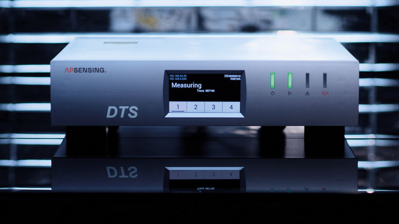
The manufacturer AP Sensing explains Raman and Brillouin approaches and the significance of strain cross-sensitivity. Its N45 series advertises a model-dependent reach up to 70 km and best-case short-range spatial resolution down to 0.5 m. Those are product claims, not universal DTS specifications and not independently benchmarked by the present lesson.

Scott Tyler (University of Nevada, Reno), Distributed Temperature Sensing Using Fiber Optics — The Basics, linked from Oregon State University CTEMPs.

Determine optical location from pulse travel time

For an idealized uniform fiber, the time delay between an outgoing laser pulse and its returned backscatter can be approximated by Δt = 2 n_g d / c. Here d is the optical distance in meters, n_g is the group refractive index, and c is the vacuum speed of light, 299,792,458 m/s. The factor of two represents the outward and return travel paths.

Assume n_g = 1.468. For a scattering location 6,000 m away, the modeled return time is 2 × 1.468 × 6,000 / 299,792,458 = approximately 58.76 microseconds. For a 2,500 m location the result is 24.48 microseconds. Other classroom distances yield 4.897 microseconds at 0.5 km and 97.934 microseconds at 10 km.

These results refer to propagation through the fiber and do not identify a point on a geographical map. Cable slack, splice trays, vault coils and changes in route can make 6 km optical distance correspond to a different surveyed ground distance. The engineering handoff must include an as-built route model, segment identifiers and the uncertainty of locating the sensor next to an actual cable or pipe.

Illustrative hotspot temperature profile

A mathematical example assigns a roughly 24°C temperature baseline to a fictional ten-kilometer sensing fiber. A Gaussian-shaped feature of 14°C amplitude is added near 6.0 km, making an approximately 38°C modeled peak. The selected width parameter is 0.25 km solely for visualization; it is not an interrogator’s measured spatial resolution.

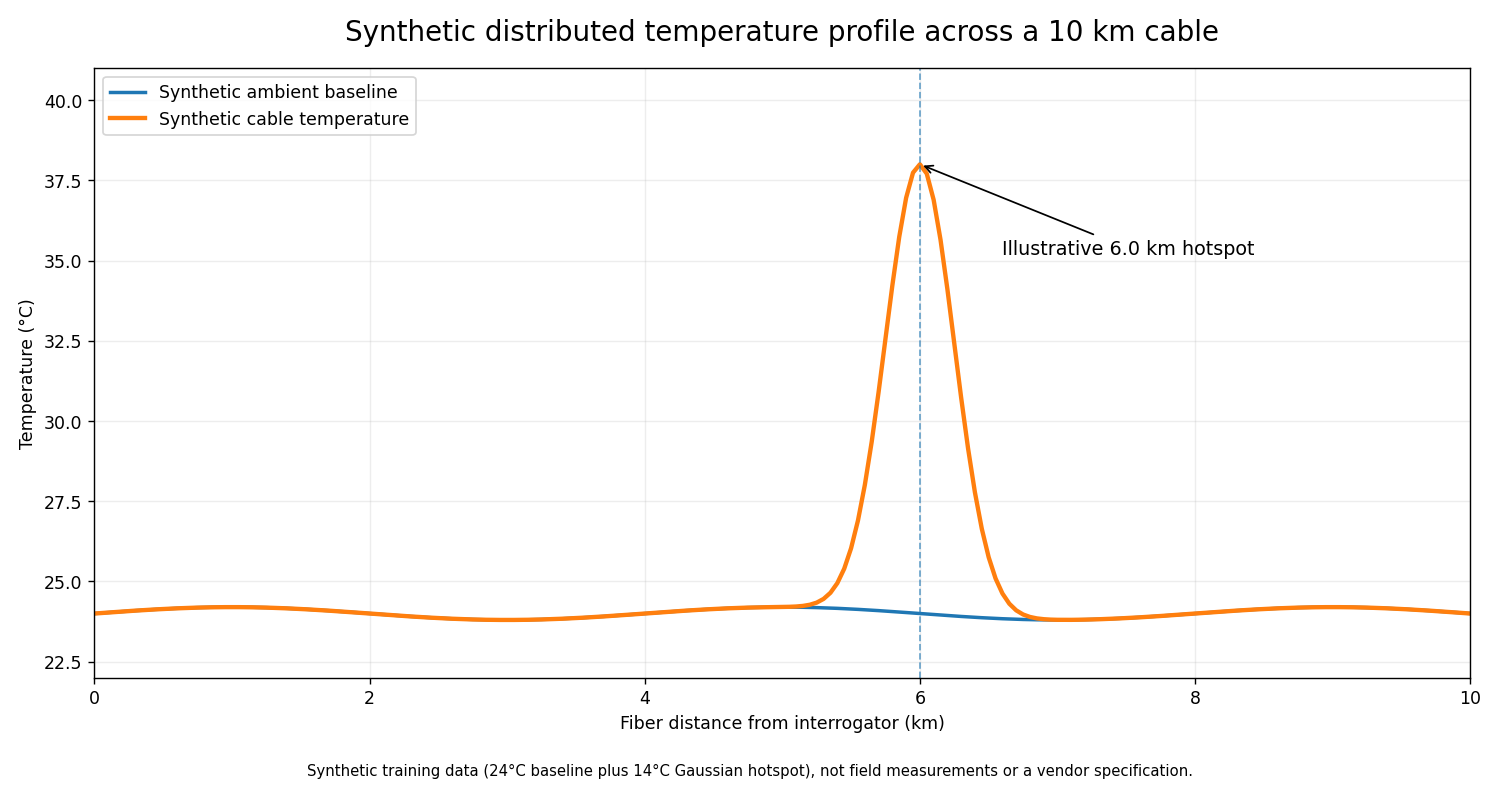
The chart is synthetic training data, not a recorded industrial fiber measurement, not a manufacturer specification, and not proof of cable overheating. Real traces respond to measurement averaging, changing optical attenuation, temperature coupling and instrument response. A sensing cable mounted outside a power cable sheath does not automatically measure the buried conductor temperature; heat-transfer modeling and field corroboration may be required.

Precision, resolution and accuracy

• **Sample spacing** is the distance between displayed temperature values. Closely spaced readings may not be statistically independent.
• **Spatial resolution** describes the minimum distance scale over which the chosen system distinguishes thermal changes under specified conditions.
• **Temperature resolution** is the smallest temperature change discernible under stated noise, time and distance averaging.
• **Accuracy** concerns agreement with a suitable calibrated thermometer, accounting for bias and uncertainty.
• **Integration time** specifies how long weak backscatter is collected. Longer averaging can improve precision but delay detection of rapid events.
• **Geographic localization** depends on actual cable geometry; even accurate optical positions may be mapped to the wrong asset.

The EPA’s educational reference notes that precision can improve with greater spatial or temporal averaging. The improvement trades against location granularity and time response. Engineers must document those choices rather than quote a single “resolution” number without a test condition.

Differential attenuation and reference calibration

Stokes and anti-Stokes photons occupy different optical wavelengths. They therefore suffer different attenuation along the sensing fiber. Raw intensity ratios can change with distance even when the cable remains at constant temperature. Splice locations, bend damage, connectors and mode coupling can introduce abrupt differences that resemble temperature features.

A defensible calibration uses reference cable sections held at known temperatures, checks independent thermometers, records the calibration interval, and estimates uncertainty due to optical loss and channel drift. Single-ended acquisition measures from one side; appropriate double-ended methods combine observations from opposite fiber ends to improve correction of some differential-attenuation effects.

The peer-reviewed open-access double-ended Raman-DTS calibration research reviews those issues. The Oregon State University CTEMPs education library also links university lectures specifically on calibration tools and practical uncertainty.

Scott Tyler (University of Nevada, Reno), DTS Calibration: Challenges and Tools, linked from Oregon State University CTEMPs.

Engineering applications and design constraints

The Electric Power Research Institute’s underground power-cable DTS application guide covers practical fiber sensing use in electrical infrastructure. Asset-monitoring applications can include underground cables, substations and industrial busways, along with pipelines and water-related environmental research. The benefit is extended spatial temperature visibility relative to sparsely placed point sensors; the cost includes sensing cable integration, mapping, commissioning, data validation and maintenance complexity.

A DTS installation is not automatically approved for fire detection or other safety-critical use. Engineering teams must select listed equipment, verify all required standards, test alarms at the system level, and document the response-time and location uncertainty. Vendor-advertised measurement range is not proof of identical accuracy and responsiveness along an entire deployed route.

Failure modes and diagnostic judgment

• A consistent offset across the trace can indicate reference-probe error, calibration drift or incorrect channel configuration.
• A step coinciding with a splice may reflect differential optical attenuation rather than an actual temperature discontinuity.
• Increased noise at long ranges may result from reduced backscatter and unsuitable averaging or pulse settings.
• A hotspot that appears to move after cable maintenance may reflect revised cable length or inaccurate route records.
• Contradictory measurements from Raman and Brillouin instruments may require a review of strain sensitivity.
• A missing history or delayed alert could originate in the telemetry network, historian or clock synchronization rather than the optical sensor.

Engineers should record which observations were directly measured, which are interpreted and which remain hypotheses. Before moving cabling or changing alert thresholds, collect trace metadata, reference temperatures, instrument identity, acquisition intervals, maintenance history and relevant independent asset readings.

Documentation-only lab

• Reproduce the optical round-trip times for 0.5, 2.5, 6.0 and 10.0 km using n_g = 1.468. Answers are 4.897, 24.484, 58.761 and 97.934 microseconds.
• Generate an illustrative 24°C baseline and an artificial 38°C peak at 6.0 km. Mark all values “synthetic” and describe the assumed spatial shape.
• A reference thermometer records 25.0°C while the interrogator shows 26.7°C. Record the discrepancy as +1.7°C and state which calibration checks should precede any correction.
• Explain why 6.0 km optical distance cannot, without route documentation, be assumed to indicate a ground location 6.0 km from the equipment room.
• Draft an engineering handoff with fiber ID, optical distance, surveyed location, uncertainty, reference calibration, alarm timestamp, measurement settings and authorized follow-up steps.

Knowledge check and answers

• **What supports temperature measurement in Raman-DTS?** A calibrated relationship between Stokes and anti-Stokes backscatter intensities.
• **What does return delay locate?** A position along the optical fiber, not automatically a geographical coordinate.
• **Why is the optical distance formula divided by two?** The measured pulse and return signal travel outward and back.
• **What is the 6 km example’s round-trip delay?** Approximately 58.76 microseconds for the assumed group refractive index.
• **Can every distributed fiber sensor separate temperature from strain?** No. The technology and compensation model matter.
• **Is 0.5 m sample spacing equivalent to 0.5 m spatial resolution?** Not necessarily.
• **Why can a splice appear to cause a temperature jump?** Stokes and anti-Stokes attenuation may differ.
• **Does a peak alone prove a physical cable fault?** No; calibration, mapping, uncertainty and corroborating evidence remain necessary.

Sources and further learning

The lesson draws on the U.S. EPA’s open DTS tutorial, the Oregon State University CTEMPs instructional library, AP Sensing’s DTS principles, the AP Sensing N45 series reference, EPRI’s openly available underground-cable application guide, and the peer-reviewed double-ended calibration research cited above. Vendor-specific specifications and safety classifications must be reviewed against the equipment actually installed.

Conclusion

Distributed fiber-optic temperature sensing links Raman physics, optical time of flight, controlled reference calibration and physical route mapping. Reliable engineering practice separates the appearance of a temperature trace from validated evidence about the asset being monitored. The synthetic calculations and chart illustrate the method without claiming field measurements or a demonstrated commercial performance result.

Editor’s Note: OSFOEC.014 follows published OSFOEC.013. The featured 1200×630 image is an original AI-generated equipment-only illustration; the in-story AP Sensing photograph is authentic manufacturer imagery. The temperature chart and timing examples are synthetic, independently calculated classroom models; no DTS or fiber hardware was tested. Educational video titles and URLs are listed by Oregon State University CTEMPs. Rendering and playback require separate checks.

On mobile, display the QR on a second screen or use your wallet’s image scanning feature. Confirm the destination and 5,000 sat amount before authorizing payment.

We volunteer daily to ensure the information on this platform is Verifiably True. If you would like to support the research, please scan the QR code.

BitcoinVersus.Tech publishes educational material; electrical, optical-laser and safety engineering decisions require qualified personnel and approved procedures.