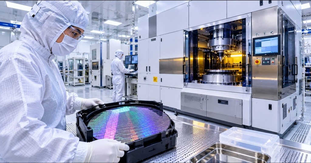
OSSEC.015 examines the lithography focus–exposure process window: the combinations of optical focus and exposure dose that print semiconductor features within an established dimensional and defect tolerance. Correct alignment of one patterned layer to another does not guarantee acceptable linewidth or resist shape. A photolithography exposure may align perfectly while printing features too wide, too narrow, incompletely developed, or distorted by defocus. Engineers therefore evaluate dose and focus together, rather than independently optimizing only one control.

The chapter follows OSSEC.014, Lithography Overlay Engineering. It also builds on OSSTC.009, Photolithography Equipment Basics and the semiconductor metrology chapter. The central educational source is the openly accessible University of California, Santa Barbara (UCSB) Nanofab focus–exposure calibration tutorial, supplemented by MIT OpenCourseWare’s Micro/Nano Processing Technology and ASML’s public technical documentation.

Learning objectives and prerequisites

• Define critical dimension (CD), exposure dose, focus offset, depth of focus, exposure latitude, process window, and focus–exposure matrix (FEM).
• Explain why a single “best-looking” die can be less valuable than a broad region of acceptable lithographic outcomes.
• Extract acceptable settings from an educational FEM and identify candidate operating points.
• Interpret the meaning and limits of a Bossung plot without presenting simulated or teaching data as experimental metrology.
• Apply the simplified Rayleigh resolution equation with consistent wavelength and numerical-aperture units.
• Recognize likely causes of CD drift and plan a documentation-only diagnostic review using real facility safeguards.

Prerequisites: basic semiconductor patterning, photoresist processing, wafer alignment, optical measurements, measurement uncertainty, and elementary algebra. An exposure tool, resist chemistry, SEM, and physical wafer are not required for the classroom exercises. Only qualified fab personnel may change scanner recipes or operate lithography hardware under site-approved procedures.

What focus and exposure control

The critical dimension is the specified width or other characteristic size of a patterned feature, often measured in nanometers (nm). Exposure dose is the light energy delivered per unit area to the resist, commonly expressed as mJ/cm² in an engineering measurement. Some equipment teaching examples label their local recipe dose with shorthand such as “mJ”; the unit reported by a particular instrument must be retained without silently converting it. Focus offset describes an intentional displacement relative to a reference focal position, often expressed in micrometers (µm).

Photolithography projects a reticle pattern onto a photosensitive material. Optics define the aerial image, while resist absorption, chemistry, post-exposure bake and development convert that optical energy into a physical feature. As focus moves away from the most suitable position, the aerial image can lose contrast or change shape. Changing dose alters the resist’s chemical response and therefore the measured CD. The direction and magnitude of CD variation depend on pattern geometry, positive or negative resist, stack reflections, numerical aperture and process chemistry. No universal rule says every feature gets wider as dose rises.

The university’s training material emphasizes that focus and exposure interact. A favorable dose at one focus setting may fail at a nearby setting. A favorable focus at one dose may fail when a photoresist coating, illumination or process variable changes. Engineers must evaluate operating margin across both axes, not merely whether a nominal test exposure succeeds.

Branch Education, “The $200M Machine that Prints Microchips: The EUV Photolithography System,” August 30, 2025. Independent educational production supported by detailed technical explanations and ASML input. Relevant portions discuss projection optics, the Rayleigh criterion, alignment and photoresist. The video is not an FEM measurement demonstration.

Focus–exposure matrices and pass/fail criteria

A focus–exposure matrix, also called an FEM or focus–exposure array, is an arranged set of exposures made with different focus and dose settings. For each exposed field, an operator or engineer assesses whether the relevant features meet the predetermined acceptance criteria. Such criteria may include printed CD tolerance, resist clearing, line continuity, profile shape, defect count, and metrology repeatability. A field that passes one dimension requirement may still fail a separate electrical or patterning requirement.

UCSB Nanofab’s public FEM tutorial shows a teaching example with eight labeled dose settings (11 through 18 mJ in its local examples) and seven focus offsets from −0.2 µm to +0.4 µm. The source identifies a contiguous pass region around its nominal settings. It recommends choosing an operating point toward the interior of the acceptable region rather than the best-looking die near a pass/fail boundary. The values are educational examples, not production data from an identified customer wafer.

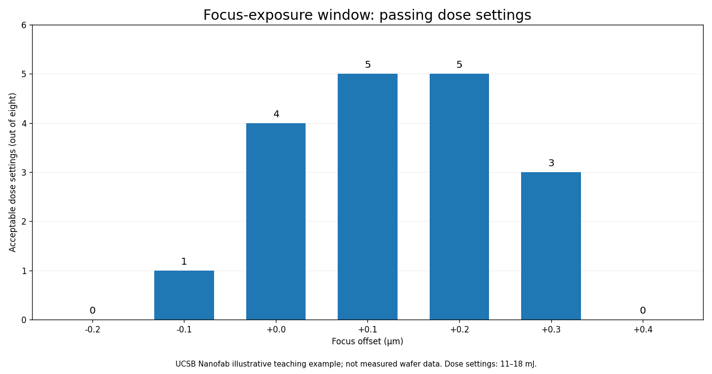
For example, the teaching table has five accepted dose settings at +0.1 µm focus and five at +0.2 µm. At the two outermost focus offsets, no listed dose setting passes. The pass count is a useful visual summary of the example’s window, but it is not a substitute for inspecting the entire two-dimensional matrix. Different rows can have the same number of passing doses while accepting different dose ranges.

The UCSB article suggests a candidate operating center of approximately 14 mJ in its example’s dose notation and +0.15 µm focus offset. Its approximate exposure and focus tolerance figures are pedagogical guidance, not guaranteed machine capability. A more precise choice requires a fine FEM, measurements of the particular pattern, a defined CD target and an explicit error budget. The coarse table cannot establish a continuous acceptance window between measured points.

Process window, exposure latitude and depth of focus

The process window is the set of focus–dose conditions meeting the chosen acceptance specifications. Exposure latitude is the dose range tolerated around a selected operating point under defined focus and process conditions; an engineer may report its absolute range, or normalize it to a nominal dose to express a percentage. Depth of focus (DOF), for a particular feature and process criterion, describes the acceptable focus span at a selected exposure dose or within a specified dose variation. DOF is not simply the physical thickness of the photoresist, and optical depth-of-focus scaling alone does not establish a manufacturing process window.

Suppose a hypothetical resist recipe is qualified from 19 to 21 mJ/cm² at the selected focus, around a 20 mJ/cm² target. Its two-sided exposure range is 2 mJ/cm². The nominal-relative deviation is ±(1/20) × 100% = ±5%; the full span is 10% of nominal. A separate hypothetical focus range from 0.00 to +0.20 µm has a span of 0.20 µm around +0.10 µm. Such arithmetic does not demonstrate that every combination of the two ranges passes: only the observed or validated joint window supports that conclusion.

How resolution and focus tolerance trade off

An often-used simplified optical-resolution expression is CD ≈ k₁ × λ / NA, where λ is the exposure wavelength, NA is numerical aperture, and k₁ aggregates many aspects of the imaging and resist process. ASML explains the relationship in its public Rayleigh-criterion teaching resource. Shorter wavelengths and larger numerical apertures can support smaller patterns, but real process performance requires calibration and advanced imaging methods.

As a mathematical example only, choosing λ = 193 nm, NA = 1.35 and k₁ = 0.35 gives CD ≈ (0.35 × 193)/1.35 ≈ 50.0 nm. The arithmetic illustrates the equation; it does not represent an independently verified feature printed on a specified scanner. Under a separate simplified depth-of-focus scaling, DOF ∝ k₂ × λ / NA², increased NA can reduce focus latitude when other factors are held fixed. The proportionality is a design heuristic, not a substitute for a measured resist process window.

If NA changes from 0.93 to 1.35 while λ and the factors are assumed fixed, the illustrative CD ratio becomes 0.93/1.35 ≈ 0.689. The idealized DOF ratio becomes (0.93/1.35)² ≈ 0.475. Both ratios are dimensionless comparisons under assumptions, not a forecast for commercial high-NA equipment. Immersion imaging, resist properties, computational corrections and application-specific constraints change practical results.

What a Bossung curve contributes

A Bossung curve presents measured or modeled critical dimension as a function of focus offset for a fixed dose. Multiple dose curves together show how critical dimension responds to the joint process variables. Flat regions may be useful because CD changes relatively little with focus; strong curvature, asymmetric response or shifts between curves may reduce usable process margin. A Bossung plot must identify its feature type, data source, dose values, focus units, metrology method and whether the traces are measured or simulated.

The UCSB Nanofab lesson teaches the acceptance-window approach from a matrix of patterned fields. For advanced study, MIT’s freely accessible micro/nanofabrication course provides foundational lithography process material. The two resources serve different purposes: one supports calibration decisions, while the other establishes the fabrication fundamentals. Neither should be presented as a measured performance report for a modern customer-specific process.

ASML, “Holistic lithography: Optimizing chipmaking from design to mass production,” June 23, 2026. Official manufacturer educational explanation of modeling, optical metrology, e-beam inspection and process control. The video provides production context; it is not a public dataset of the UCSB FEM example.

How focus and dose excursions affect yield

Excess exposure variation can shift patterned dimensions away from their target; an unacceptable CD can contribute to timing, leakage, contact resistance or pattern-transfer errors depending on the feature. Focus errors can reduce optical contrast and create defects, resist-profile problems or bridging and breaks. A scanner can still have acceptable overlay while the printed dimensions are outside control limits. The preceding overlay engineering lesson explains the positional error axis, while OSSEC.012 on yield and defect density explains why several independent defects can affect an overall yield calculation.

Focus and dose variations may be affected by scanner performance, wafer height maps, substrate topography, coating thickness, bake drift, alignment history, optics, reticle patterns and wafer-to-wafer differences. Root-cause analysis should correlate metrology, sensor status, maintenance changes and wafer maps rather than attributing every CD excursion to the exposure source alone. The semiconductor statistical process-control chapter describes how time trends and capability metrics help identify process shifts without confusing observed correlation with proven causation.

A disciplined engineering workflow

1. Establish the specification. Identify the CD target, acceptable range, defect limits, feature geometry and applicable measurement uncertainty. Document substrate stack and resist processing, not only scanner settings.
2. Validate the data source. Determine whether a matrix contains measured CDs, simulation, published educational pass/fail examples or production qualification records. Do not merge those evidence categories.
3. Inspect all dimensions of the matrix. Find contiguous passing regions in both dose and focus, and identify boundaries where additional test exposures may be required.
4. Choose margin rather than an isolated optimum. Prefer a setting with verified tolerance to ordinary process variation. A single successful die on a boundary does not demonstrate a robust recipe.
5. Validate nearby conditions. Use a finer matrix and repeated metrology where authorized. Check for differences among fields, wafers, feature orientations and process stages.
6. Assess the full process chain. Include resist preparation, coating, exposure, baking, development and downstream pattern transfer, with contamination and tool safety controls.
7. Record decision and residual uncertainty. Store process window boundaries, instrument and recipe identifiers, dates, acceptance metrics, review approvals and unresolved issues.

A university teaching example is not a tool qualification recipe. In a real laboratory, sample preparation, solvent exposure, laser safety, chemical handling, electrical systems and expensive exposure equipment require training and facility authorization. The UCSB ASML Stepper SOP is a tool-specific educational reference, not permission to operate hardware at another institution.

Documentation-only lab: reading the UCSB matrix

1. Open the UCSB Nanofab FEM tutorial and copy the example’s seven focus offsets and eight dose-column labels to a notebook or spreadsheet. Keep the source’s shorthand dose notation, and separately note that physical radiant exposure is commonly specified per unit area.
2. Mark a field as 1 if the university example labels it within tolerance and 0 otherwise. Count passing settings in each focus row. Confirm the sequence 0, 1, 4, 5, 5, 3, 0 shown in the bar chart.
3. Compare the +0.1 and +0.2 µm rows. Both have five passing doses, but the accepted columns matter more than their count alone. Locate an overlapping interior set of acceptable dose/focus combinations.
4. Explain why +0.15 µm is only an approximate interpolated focus center when the chart and source matrix sample discrete 0.1 µm steps. Propose an authorized finer experiment that would check the interpolation.
5. Calculate the hypothetical Rayleigh CD using λ = 193 nm, NA = 1.35 and k₁ = 0.35. State the assumptions and distinguish the calculated ~50.0 nm from a measured critical dimension.
6. Prepare a one-paragraph engineering review: which operating point would be considered, what evidence supports it, which constraints are unresolved, and which qualified metrology steps must precede any production approval.

Knowledge check with explained answers

1. Why are focus and dose analyzed together? Both influence aerial-image and resist outcomes, so a setting acceptable for one dose may fail at another focus.
2. What does a focus–exposure matrix show? A set of exposed fields with varied focus and dose, classified or measured against defined feature specifications.
3. What is the process window? The combination of settings that meet the chosen quality criteria, not a universal machine rating.
4. Why can a single “best die” be a poor recipe choice? It may be close to a failure boundary and have little margin for normal variation.
5. What does the UCSB teaching bar chart show at +0.1 µm? Five acceptable dose settings from its eight labeled columns; the example is not a measured production experiment.
6. What is the nominal-relative dose tolerance from 19 to 21 mJ/cm² around 20 mJ/cm²? ±5% around nominal; 10% is the total span as a fraction of nominal.
7. Does CD ≈ k₁λ/NA guarantee a printed CD? No. It is simplified imaging guidance and omits important process-specific effects.
8. What does a Bossung curve plot? CD versus focus at a fixed dose; multiple curves can compare several doses.
9. Does passing a CD test prove acceptable overlay? No. CD and overlay are different dimensions of patterning quality.
10. Can an open university tutorial be used as an unmodified fab operating procedure? No. Site-authorized procedures and equipment-specific safety requirements are mandatory.

Open educational sources and technical references

UCSB Nanofab Wiki, “Lithography Calibration — Analyzing a Focus-Exposure Matrix” (open university teaching resource, October 22, 2024); UCSB Nanofab tutorial index; MIT OpenCourseWare, 6.152J Micro/Nano Processing Technology; ASML, Rayleigh Criterion for Resolution; ASML, Lithography Principles; and ASML, Lenses and Mirrors. The cited university and manufacturer resources are used for education and technical context; the original teaching chart retains its stated limitations.

Conclusion

A viable lithography recipe is not simply an exposure with the sharpest-looking feature. It requires a defensible acceptance window in dose and focus, correctly interpreted metrology, documented uncertainty and sufficient operating margin. An FEM identifies candidate regions, Bossung analysis characterizes CD response, and qualified engineering validation determines whether the process is stable enough for its intended application. The next curriculum subject is determined from live WordPress and GitHub inventory, not from an assumed topic sequence.

Editor’s Note: OSSEC.015 follows the confirmed OSSEC.014 chapter. Technical explanations draw primarily on the open UCSB Nanofab training wiki, MIT OpenCourseWare and ASML. The illustrated bar chart is independently plotted from UCSB’s educational pass/fail example; it is not experimental fab data. The featured cover is original, photorealistic AI editorial imagery, and the in-story cleanroom photograph is from ASML. No custom schematic or conceptual diagram was produced. Arithmetic examples were checked separately; no lithography tool was operated, wafer exposed or CD measured for the article. Both videos were verified against their publisher descriptions. Live video playback and visual responsive rendering are audited separately.

To scan the 5,000-sat donation QR on a phone, open the article on a separate screen and scan with a compatible Bitcoin wallet, or use a saved-image scan in wallets supporting that feature. Confirm the destination before paying.

We volunteer daily to ensure the information on this platform is Verifiably True. If you would like to support the research, please scan the QR code.

BitcoinVersus.tech provides educational and journalistic information and is not a financial advisor.