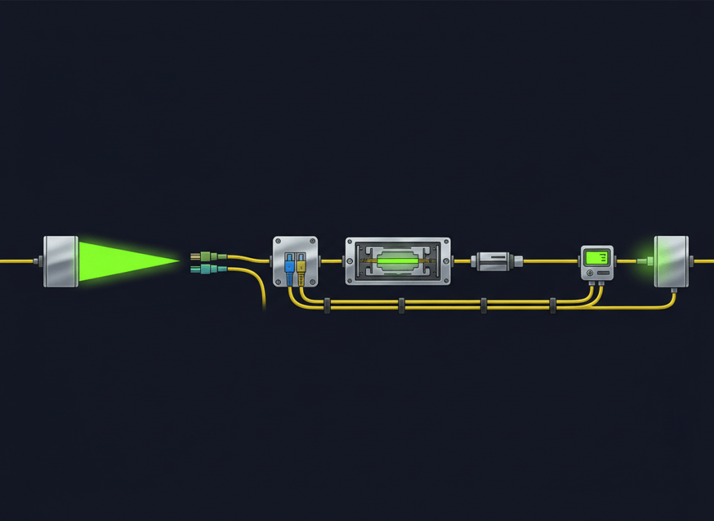
A fiber link is not engineered by asking whether light reaches the far end. It is engineered by proving that the receiver gets enough optical power under worst-case conditions—without being overloaded—and that enough margin remains for aging, contamination, repair, measurement uncertainty, and real-world variation.
This is OSFOEC.001, the first lesson in the Open Source Fiber Optics Engineer Certification track. It builds on OSFOTC.001: Fiber Optic Safety, Handling, Inspection, and Cleaning Basics and moves from technician handling discipline into link-level engineering: dB, dBm, transmitter/receiver limits, cable-plant loss, design margin, overload checks, dispersion penalties, and acceptance criteria.
The link-budget model
transmitter output
↓ subtract fiber attenuation
↓ subtract mated-connection loss
↓ subtract splice loss
↓ subtract splitter / passive-device loss
↓ subtract engineering reserve and penalties
↓
receiver input power
The basic received-power equation is:
PRX (dBm) = PTX (dBm) − total optical loss (dB) + optical gain (dB)
If there are no optical amplifiers, the gain term is zero.
1. dBm is absolute power; dB is a ratio
dBm expresses absolute optical power referenced to 1 milliwatt. dB expresses a relative gain or loss ratio.
- 0 dBm = 1 mW.
- +3 dBm is approximately 2 mW.
- −3 dBm is approximately 0.5 mW.
- A 3 dB loss cuts optical power roughly in half.
- A 10 dB loss reduces power to one-tenth.
This matters because engineers add and subtract optical losses in dB while transmitter and receiver specifications are usually expressed in dBm.
Video 1: The mysterious dB of fiber optics
2. Power budget and loss budget are related—but not identical
The Fiber Optic Association separates two terms that are often confused:
- Power budget: the amount of optical loss the transmitter/receiver pair can tolerate while still meeting the required performance.
- Loss budget: the estimated loss of the passive cable plant based on fiber length, connections, splices, splitters, and other passive components.
See FOA’s loss-budget engineering reference and its fiber-optic data-link reference.
The design condition is simple:
allowable power budget must exceed expected cable-plant loss plus required margin and penalties.
3. Calculate maximum allowable loss from the transceiver limits
For a simple digital link, the worst-case maximum allowable path loss begins with the minimum guaranteed transmitter output and the receiver sensitivity.
Maximum allowable loss = minimum transmitter output − receiver sensitivity
Example:
minimum transmitter output = −2 dBm
receiver sensitivity = −15 dBm
maximum allowable loss = −2 − (−15)
= 13 dB
That 13 dB is not automatically available for cable alone. Engineering reserve, dispersion-related penalties, aging, implementation penalties, and specification requirements may consume part of it.
4. Estimate cable-plant loss component by component
A practical passive-link estimate is:
Total loss = fiber loss + connection loss + splice loss + passive-device loss
Fiber loss is:
fiber attenuation coefficient (dB/km) × link length (km)
The attenuation lesson covers the physical meaning of optical power reduction, while insertion loss covers measured loss introduced by a component or complete link.
Video 2: Loss budgets
5. Worked example: 10 km singlemode link
Assume this simplified design example:
- minimum transmitter output: −2 dBm
- receiver sensitivity: −15 dBm
- fiber length: 10 km
- design fiber attenuation: 0.35 dB/km
- four mated connections: 0.5 dB each
- two fusion splices: 0.1 dB each
- engineering reserve: 3 dB
Step 1 — transceiver power budget
−2 − (−15) = 13 dB
Step 2 — fiber loss
10 km × 0.35 dB/km = 3.5 dB
Step 3 — connection loss
4 × 0.5 dB = 2.0 dB
Step 4 — splice loss
2 × 0.1 dB = 0.2 dB
Step 5 — expected passive loss
3.5 + 2.0 + 0.2 = 5.7 dB
Step 6 — raw optical margin
13 − 5.7 = 7.3 dB
Step 7 — reserve 3 dB
7.3 − 3 = 4.3 dB remaining design margin
The arithmetic is easy. The engineering work is choosing defensible worst-case values for wavelength, temperature, fiber type, connector population, splice plan, transceiver tolerances, expected restoration events, aging, and required reliability.
6. Use guaranteed worst-case values—not convenient typical values
Typical component performance is useful for understanding a design, but production acceptance should be tied to applicable standards, customer requirements, manufacturer data, and the actual transceiver specification.
When selecting optics, engineers should examine:
- minimum and maximum transmitter output;
- receiver sensitivity at the required BER;
- maximum receiver input / overload limit;
- wavelength range;
- supported fiber type;
- temperature grade;
- maximum specified reach;
- dispersion tolerance or penalty;
- FEC assumptions;
- connector or reflectance constraints where specified.
7. Always perform the overload check too
A link can fail because received power is too low, but some receivers can also be overloaded by too much optical power.
Suppose:
maximum transmitter output = +1 dBm
maximum safe receiver input = −1 dBm
The path needs at least:
+1 − (−1) = 2 dB of loss
If the real path loss were only 1 dB, the receiver could exceed its specified maximum input and an optical attenuator might be required. FOA’s loss-budget guidance specifically notes that links can have both minimum- and maximum-loss requirements.
8. Measure power with the correct wavelength and reference
The optical power meter is the fundamental instrument for measuring transmitter output and received optical power. Measurement quality depends on the correct wavelength setting, compatible detector range, clean adapters, known-good reference cords, and a documented reference method.
Do not confuse a live received-power reading with a complete cable-plant insertion-loss test. They answer related but different questions.
9. Measurement uncertainty belongs in the engineering decision
Every optical measurement has uncertainty. Connector repeatability, source stability, detector calibration, reference-cord quality, mode distribution, wavelength, and test setup can all move the measured result.
FOA’s current 2025 fiber-optic installation standard treats the loss budget as a design estimate that should also guide post-installation acceptance testing. Engineers should not create a pass/fail threshold so tight that normal measurement uncertainty causes good links to fail—or hides bad links behind unrealistic assumptions.
10. Dispersion can limit reach even when optical power is adequate
A pure attenuation calculation is not enough for high-speed or long-reach links. Dispersion spreads optical pulses in time and can close the receiver eye even when the received power is numerically above sensitivity.
- Modal dispersion: a major bandwidth limit in multimode fiber.
- Chromatic dispersion: different wavelengths travel with different group velocities.
- Polarization-mode dispersion: polarized components of the signal can experience different delays in singlemode fiber.
The polarization-mode dispersion (PMD) lesson and fiber characterization lesson connect directly to this engineering limit.
FOA’s data-link reference notes that dispersion can reduce the usable power budget because pulse distortion imposes an additional performance penalty.
Video 3: Attenuation in a fiber-optic link
11. FEC helps digital performance, but it is not “free optical power”
Forward error correction can allow a digital system to meet its target BER at a lower pre-FEC signal quality than an uncoded system, but engineers should use the transceiver standard and datasheet limits exactly as specified. Do not arbitrarily add “FEC gain” to an optical budget unless the link specification explicitly defines how that margin is accounted for.
12. Splitters, WDM filters, muxes, and passive optics consume budget
Any passive optical element can add insertion loss:
- splitters and taps;
- CWDM/DWDM mux/demux filters;
- MPO/MTP connection pairs;
- patch panels and cassettes;
- optical circulators;
- isolators;
- monitor taps;
- attenuators.
The splitters vs. taps lesson is a useful precursor. Later OSFOEC lessons extend this into CWDM/DWDM channel planning, coherent links, amplifier chains, OSNR, and nonlinear effects.
13. Design margin has a job
Margin is not an arbitrary comfort number. It exists to absorb uncertainty and degradation that were not explicitly modeled as deterministic losses.
- source aging;
- connector contamination or remating variation;
- future restoration splices;
- temperature variation;
- manufacturing tolerance;
- measurement uncertainty;
- minor route changes;
- component replacement variance.
FOA commonly uses several decibels of excess margin in example designs, but the correct reserve depends on the application and the governing equipment/standard requirements. Do not blindly apply one universal number.
14. Engineer from both ends of the specification
A robust optical design checks at least two extreme cases:
- Minimum-power case: minimum TX output, maximum expected path loss, penalties, and required margin must still leave the receiver at or above sensitivity.
- Maximum-power case: maximum TX output and minimum possible path loss must not exceed receiver overload.
For temperature-sensitive or wavelength-sensitive systems, repeat the calculation at the relevant environmental and spectral corners.
15. Acceptance testing should map back to the design
The design budget should become an acceptance criterion. If the engineered passive loss is 5.7 dB, the installation team should know what measured result is expected, what test method applies, what uncertainty is allowed, and when a high-loss link requires segment-by-segment troubleshooting.
This closes the loop:
design → install → inspect/clean → measure → compare to budget → troubleshoot exceptions → document final as-built loss
16. Engineer’s link-budget checklist
- Identify the exact transceiver standard and part specification.
- Record minimum and maximum TX output.
- Record receiver sensitivity and maximum receiver input.
- Confirm wavelength and fiber type.
- Measure or document route length.
- Count every mated connection.
- Count every planned splice.
- Include splitters, muxes, taps, attenuators, or other passives.
- Use defensible attenuation and component-loss values.
- Calculate expected passive loss.
- Subtract explicit implementation/dispersion penalties if required.
- Add the required engineering reserve.
- Check the minimum-power case.
- Check the maximum-power / overload case.
- Define the acceptance-test method and uncertainty.
- Record the final as-built and measured values.
Practice exercise
A transceiver pair has minimum TX output of −1 dBm and receiver sensitivity of −13 dBm. The planned link contains 8 km of fiber at 0.35 dB/km, six mated connections at 0.4 dB each, and four splices at 0.1 dB each.
- Calculate the transceiver power budget.
- Calculate total fiber loss.
- Calculate connection loss.
- Calculate splice loss.
- Calculate total expected passive loss.
- Calculate raw optical margin.
- If the project requires 3 dB reserve, how much margin remains?
- What additional information is still needed to check receiver overload?
Answer check: power budget = 12 dB; fiber = 2.8 dB; connections = 2.4 dB; splices = 0.4 dB; expected passive loss = 5.6 dB; raw margin = 6.4 dB; remaining after 3 dB reserve = 3.4 dB. The overload check still requires maximum TX output and maximum allowed receiver input.
Knowledge check
1. What is the difference between dB and dBm?
dB is a relative gain/loss ratio; dBm is absolute power referenced to 1 milliwatt.
2. What is the transceiver power budget?
The optical-loss range the transmitter/receiver pair can tolerate, derived from transmitter output and receiver input requirements.
3. What is the cable-plant loss budget?
The estimated passive loss of fiber, mated connections, splices, splitters, and other passive components.
4. Why check receiver overload?
Because a very short or low-loss link can deliver more optical power than the receiver is specified to accept.
5. Can a link pass its attenuation budget and still fail at high speed?
Yes. Dispersion and other signal-quality penalties can limit reach even when received optical power is adequate.
6. Why use design margin?
To absorb aging, contamination, future repair, tolerance, environmental variation, and measurement uncertainty not otherwise modeled.
Key takeaway
Optical engineering is a bounded power problem. Start with guaranteed transmitter and receiver limits. Calculate passive loss. Account for penalties and margin. Check both low-power and overload corners. Then connect the design budget to the field acceptance test.
Engineering note: The numeric examples in this lesson are illustrative, not universal design limits. Real links must use the exact transceiver specification, fiber/cable data, passive-component specifications, applicable standards, environmental limits, required BER/FEC conditions, and project acceptance criteria.
BitcoinVersus.Tech
Advertisement
Editor’s Note:
We volunteer daily to ensure the credibility of the information on this platform is Verifiably True. If you would like to support our research initiatives, please donate here: 3C9o19EH5HSiwEPyCTmEKzxhNCbo2X6TTb
BitcoinVersus.tech is not a financial advisor. This media platform reports on financial subjects purely for informational purposes.


Leave a Reply