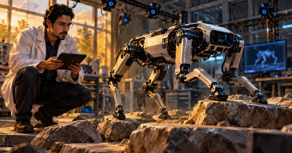
Robot state estimation is the process of inferring a robot’s internal motion and position from imperfect measurements. A controller may know how fast it commanded a wheel or joint to move without knowing exactly where the machine ended up. Wheel slip, sensor noise, calibration error and external forces create differences between predicted motion and actual motion. An estimator addresses this problem by combining a mathematical motion model with available observations. Kalman filtering provides one mathematical framework for repeatedly updating the estimate and its uncertainty; its extended variant (EKF) is widely used where motion and sensor relationships are nonlinear. This subject builds on robot feedback control, robot velocity kinematics and control barrier functions.

Elementary Overview

Imagine a robot traveling across a room without being allowed to look at the floor all the time. Its wheels can report how far they turned, but the wheels might slip. A camera can see the surroundings, but images can be blurry. A motion sensor can detect turning, yet tiny errors accumulate. No single instrument gives a perfect answer.

A state estimator is the robot’s method for combining these clues. It starts with a prediction of where the robot should be, checks measurements of where it appears to be, and combines the two based on how much each can be trusted. The estimator also reports how uncertain its answer is. That uncertainty helps engineers decide whether a measurement or controller action deserves confidence.

What Counts as a Robot State?

A state vector is a collection of variables sufficient for the chosen motion model. A two-dimensional mobile robot might have position x and y, heading angle θ, forward speed v and angular speed ω. A manipulator might track joint positions and joint velocities; an inertial navigation filter can include accelerometer and gyroscope biases. The state vector’s structure is a modeling decision, not a universal inventory of all robot properties.

State variables are not always measured directly. A wheel encoder reports rotation, from which displacement can be estimated with wheel diameter and gearing assumptions. An inertial measurement unit (IMU) reports angular rate and specific force, not absolute position. A camera or lidar may provide relative pose constraints, while GNSS, when available and usable, can contribute position information. Correct use of a vision calibration is essential before camera-derived measurements are fused with motion estimates.

Uncertainty and the Covariance Matrix

An estimate is commonly written as x̂ and its uncertainty as a covariance matrix P. In a simple one-dimensional model, P is just a nonnegative variance measured in the square of the position unit. The square root of variance is the standard deviation. For a multi-variable system, the diagonal of P contains variances and off-diagonal terms describe correlations between state-estimation errors.

Covariance is not a direct certificate that the state is correct. It is a statistical characterization conditional on assumptions about the model, sensor errors and data association. An overconfident filter can report small covariance while tracking the wrong position. Engineers check both estimated accuracy and consistency against independent ground truth where available, especially after changing sensor hardware, coordinate frames or dynamics.

The Kalman Filter Prediction Step

For a linear discrete-time model, a conventional Kalman filter predicts x̂_k|k−1 = A x̂_k−1|k−1 + B u_k. Here A advances the modeled state, B maps known controls into the state, and u is the control input. The corresponding covariance prediction is P_k|k−1 = A P_k−1|k−1 Aᵀ + Q, where Q represents process-noise covariance.

The prediction step models what should happen between measurements. Even when motor commands are known, unexpected wheel slip or contact forces can make that model uncertain. Increasing Q describes greater uncertainty in modeled evolution; it is not a generic fix for a poorly calibrated sensor. MIT’s state-estimation notes place observers and Kalman filtering within robotics control and distinguish them from recursive Bayesian methods more generally.

The first university lecture explains how prediction and feedback correction produce a state estimate. Note the different roles of motion uncertainty and measurement uncertainty rather than assuming one input must always dominate.

Measurement Updates and Kalman Gain

Suppose a sensor reports a measurement z related to the state by a matrix H. The innovation is y = z − H x̂_prior. The innovation covariance is S = H P_prior Hᵀ + R, where R is measurement-noise covariance. Provided S is invertible, the Kalman gain is K = P_prior Hᵀ S⁻¹, and the corrected estimate is x̂_posterior = x̂_prior + K y.

A small measurement-noise covariance R relative to predicted uncertainty tends to give a valid measurement more influence, while a large R generally limits its influence. This interpretation relies on the errors having correctly modeled statistics and on the measurement corresponding to the intended physical quantity. For numerical robustness, the Joseph covariance update P_posterior = (I−KH)P_prior(I−KH)ᵀ + KRKᵀ is often preferred to a simplified covariance formula.

Worked Example: Combining Two Position Estimates

Consider a stationary snapshot of a robot along one axis. Its predicted position is 1.0 m with variance 0.16 m² (standard deviation 0.4 m). A separate position sensor reports 1.6 m with variance 0.09 m² (standard deviation 0.3 m). Under independent, unbiased, Gaussian error assumptions, the scalar gain is K = 0.16 / (0.16 + 0.09) = 0.64. The innovation is 0.6 m, so the corrected estimate is 1.0 + (0.64 × 0.6) = 1.384 m.

The posterior variance is (1 − 0.64) × 0.16 = 0.0576 m², corresponding to a standard deviation of 0.24 m. The estimate moves toward the measurement because the latter was modeled as more precise, but does not simply replace the prediction. The result is hypothetical and depends critically on the validity and independence of the uncertainty assumptions. Two sensors affected by the same miscalibration cannot be treated as independent measurements without correction.

Nonlinear Robots and the Extended Kalman Filter

Real robots do not always obey linear motion models. For a turning mobile robot, position changes are related to the sine and cosine of its orientation. An extended Kalman filter (EKF) handles nonlinear models by predicting with a nonlinear transition function x_k = f(x_k−1, u_k) and predicting sensor observations with z_k = h(x_k). It evaluates Jacobians of those functions near the current estimate to propagate covariance and calculate corrections.

The EKF is not guaranteed to recover from large model errors, incorrect initial orientation or inconsistent measurements. Linearization can become inaccurate when uncertainty is broad or nonlinearities are strong. Other options include unscented Kalman filters, particle filters, factor-graph optimization and smoothing, selected according to the application and computational budget. The ROS 2 robot_localization package provides extended and unscented Kalman filter nodes; its maintainer documentation distinguishes the two prediction approaches.

University Example: Estimating an Inverted Pendulum

The second lecture applies Kalman filtering in MATLAB to an inverted pendulum on a cart. The physical system differs from a mobile robot, but the same prediction-versus-measurement logic applies to robot velocity and orientation estimation. The lecture is useful for seeing covariance and gain in a state-space implementation rather than as abstract symbols alone.

Timing, Frames and Sensor Correlation

Robotic sensor fusion fails easily when measurements are expressed in different frames or assigned the wrong times. Wheel odometry may be expressed relative to odom, a robot body to base_link, and a global localization system to map. A pose estimate in one frame cannot be mixed with values in another without the appropriate transform. Encoder, IMU and camera data must also be timestamped consistently; using an old camera pose as if it were current can create a position jump even when the filter mathematics is correct.

An estimator should avoid double-counting correlated data. For example, a robot’s odometry message may already incorporate an IMU; fusing both that message and the same IMU measurement as independent data exaggerates confidence. The navigation stack’s robot_localization configuration guide illustrates publishing a filtered odometry estimate and using frame transforms within ROS 2. Its example should be adapted to the actual robot and software distribution, not copied blindly into a production system.

Observability, Residuals and Diagnostic Evidence

A state is observable when the available measurements and motion model contain enough information to distinguish it from other possible states. An encoder and gyroscope may estimate short-term motion without revealing absolute position in a building. Without an external reference or informative environment observations, position drift can accumulate even when velocity estimates look stable. An estimator cannot manufacture missing information simply by tuning covariance matrices.

Engineers assess innovation residuals, time synchronization, state-estimate discontinuities, measurement rejection counts and covariance trends. A persistent biased residual suggests incorrect calibration, model parameters or a frame mismatch. Rapidly increasing uncertainty may be appropriate when observations disappear; suspiciously low uncertainty in that situation can reveal overconfident noise parameters. The purpose of statistical monitoring is to identify model and sensor problems before those estimates mislead robot motion controllers.

Read-Only Robot State Estimation Lab

In an offline or authorized ROS 2 environment with the relevant nodes already running, inspect the available measurement stream, filtered odometry and transforms. The commands ros2 topic list, ros2 topic echo /odometry/filtered --once and ros2 run tf2_ros tf2_echo odom base_link are examples; actual topic and frame names can differ, and the second command only returns if that topic exists and supplies data. These are observational diagnostics, not a procedure for modifying a live robot.

• Record the robot model, software version, operating state, sensors, message timestamps and coordinate-frame conventions.
• Check which sensors supply position, orientation, velocity and angular velocity, and whether any already contain fused measurements.
• Compare raw measurement sequences with the estimator output across a known test interval and note missing, delayed or out-of-order messages.
• Examine state uncertainty and residual trends against independently obtained reference measurements where possible.
• Document suspected calibration, timestamp or covariance issues and route changes through approved simulation and validation procedures.

Safety and Reliability Boundaries

State estimates can fail in ways that produce plausible-looking numbers. Localization loss, bad GNSS conditions, camera occlusion, wheel slip and IMU bias should be included in a risk assessment. Neither a Kalman filter nor a low reported covariance is a substitute for independently engineered protective functions, guarding, emergency-stop systems or validated motion limits. The principles in control barrier functions likewise depend on assumptions about the state and dynamics; corrupted estimates can invalidate those assumptions.

Knowledge Check

• What is the difference between a state measurement and a state estimate?
• Why does process-noise covariance Q appear in the prediction step?
• For predicted variance 0.16 m² and measurement variance 0.09 m², what is the scalar Kalman gain?
• Why does the EKF require Jacobians of nonlinear transition or observation functions?
• Why can fusing IMU data twice create an overconfident estimate?
• What observations distinguish a frame mismatch from a sensor that simply has more random noise?

Answers: A measurement is a sensor observation; an estimate combines observations and model predictions. Q represents uncertainty in state evolution not captured by the nominal dynamics. The scalar gain is 0.64. Jacobians approximate how nonlinear models change near the current estimate so covariance can be propagated. Duplicate correlated inputs are incorrectly treated as independent evidence. A frame mismatch can produce persistent structured offsets or orientation-dependent residuals, while higher random noise more commonly increases scatter; independent tests are necessary to distinguish them.

Elementary Conclusion

A robot cannot directly know every detail of its movement. Sensors provide pieces of information, and a motion model predicts what should happen between those readings. A Kalman filter uses both to produce an estimate of position or motion and a numerical description of how uncertain the estimate may be.

Good robotics engineering does not stop at obtaining a smooth number. It checks that sensors agree on time, use the same reference frames and have realistic uncertainties. These checks make the robot’s estimated state more useful to navigation, manipulation and safety-related engineering.

Primary References and Related Lessons

The technical foundation includes MIT Underactuated Robotics: State Estimation, ROS 2 robot_localization package, ROS state estimation node documentation, and the Navigation2 filtered-odometry setup guide. Related BitcoinVersus.Tech chapters cover feedback control, velocity kinematics, vision calibration, and control barrier functions.

BitcoinVersus.Tech Editor’s Note: We volunteer daily to ensure the credibility of the information on this platform is Verifiably True. If you would like to support our work and help further secure the integrity of our research initiatives, please scan the QR code below to donate 5,000 sats.

For mobile-wallet scanning, display the QR code on a laptop or larger screen and scan it using your phone. Verify the recipient Bitcoin address before sending funds.

BitcoinVersus.tech is not a financial advisor. This media platform reports on financial subjects purely for informational purposes.