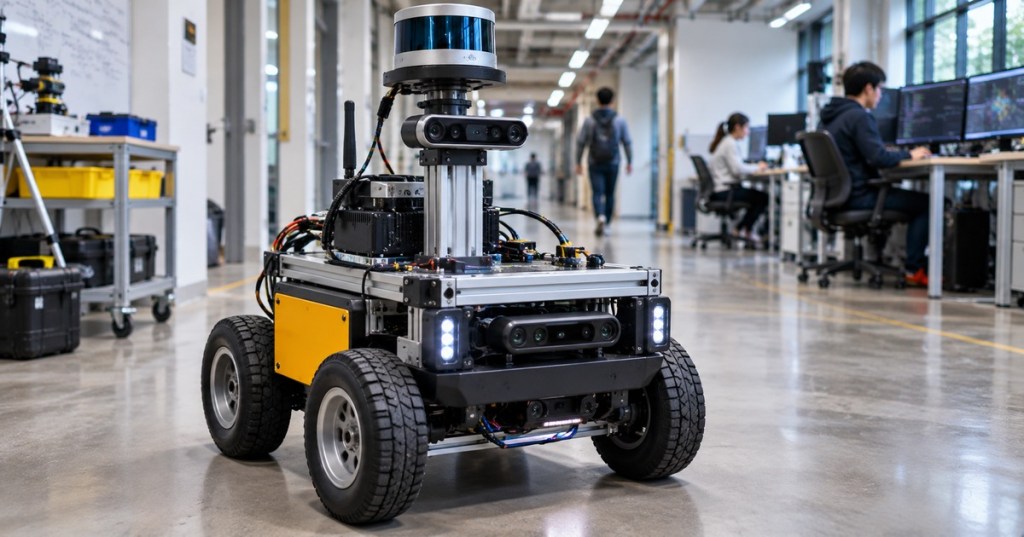
OSREC.014 introduces pose-graph simultaneous localization and mapping (SLAM), a method for estimating a mobile robot’s trajectory by jointly reconciling uncertain motion measurements and revisits to known places. Wheel encoders and inertial estimates drift as a robot moves; cameras or LiDAR can supply new geometric constraints when the robot recognizes a location again. A graph optimizer adjusts multiple earlier poses together, rather than merely correcting the latest position. This lesson continues OSREC.013 on Kalman filtering and uncertainty and extends individual state estimation into global trajectory consistency.

Learning Objectives and Prerequisites

• Describe a pose, motion constraint, prior factor, loop closure, and measurement covariance.
• Explain why odometry drift accumulates and how a valid loop closure can constrain older estimates.
• Distinguish graph construction, loop-closure detection, robust estimation, and optimization.
• State the weighted least-squares objective and the significance of measurement uncertainty.
• Reproduce a small numeric example using Python and verify its output.
• Identify false loop closures, gauge freedom, poor initialization, and inconsistent sensor timestamps.
• Explain the difference between a demonstration using synthetic measurements and a tested production SLAM deployment.

Prerequisites: coordinate frames and transforms, robot odometry, basic vectors and matrices, probability, and Python fundamentals. Review robot Jacobians, inverse kinematics, and the earlier state-estimation lesson as needed. The documentation-based lab requires Python 3 with NumPy; operating a real mobile robot is neither required nor authorized by the example.

Elementary Overview: Why Returning to the Same Place Matters

Imagine a wheeled robot that drives several meters around a room and eventually returns to its starting point. Its wheels report the distance they rotated, but small slips make the inferred path fail to close. The map may appear stretched or bent. If a LiDAR scan or a camera confidently recognizes the starting location, the robot has obtained a new observation connecting an earlier visit to its current position. The optimizer can distribute the correction over the trajectory according to the reliability of its measurements.

A loop closure is a constraint from place recognition and geometric verification, not simply an instruction to reset the latest position to zero. Some apparent matches are false, especially in symmetric corridors, warehouse aisles, or repeated shelving. A bad match can deform the entire map, making validation and robust residual handling essential.

MathWorks/MATLAB official educational video, “Understanding SLAM Using Pose Graph Optimization | Autonomous Navigation, Part 3,” published July 8, 2020 on YouTube. Explains accumulated uncertainty, pose constraints and optimization. Source: verified MATLAB channel; software instruction rather than footage of the lesson’s synthetic experiment.

What Is in a Pose Graph?

A pose represents a robot’s position and orientation at a selected instant. A planar pose can be written as (x, y, θ); full spatial pose commonly involves a 3D position and 3D rotation. Nodes correspond to unknown poses. Factors describe observations that constrain one or more nodes: an initial pose prior, wheel-odometry transforms, scan-matching results, or a loop closure. An optimizer finds pose values that best reconcile the factors.

In GTSAM’s official open-source Pose2 SLAM tutorial, a PriorFactorPose2 anchors the first pose, while BetweenFactorPose2 connects successive poses and closes a loop to an earlier pose. The project distributes practical examples and documentation as part of the GTSAM tutorial. The principle is independent of whether measurements arrive from a wheel encoder, visual odometry, LiDAR matching, or another calibrated sensor pipeline.

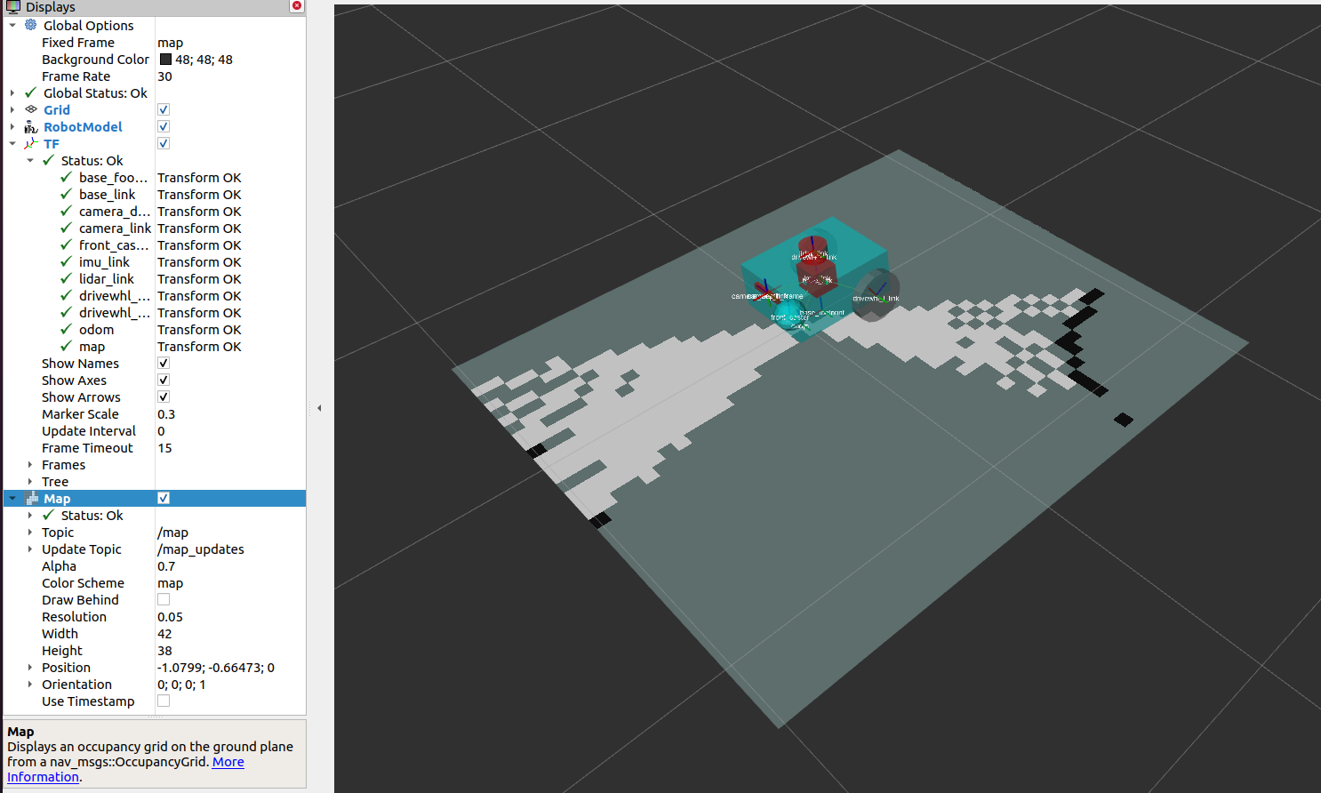
The graph structure is not the occupancy map itself. Graph optimization estimates poses; an occupancy-grid system may then transform individual LiDAR scans using the corrected poses to update the map. The open-source ROS 2 SLAM Toolbox package provides mapping, pose-graph serialization and localization capabilities. Its actual message interfaces and transforms must be interpreted using the selected ROS distribution’s documentation, not by assuming that every SLAM package has identical behavior.

The Optimization Objective and What the Weights Mean

For a collection of constraints, an optimizer compares each measured relative transform with the relative transform implied by its current pose estimates. The difference is called a residual. A standard maximum-likelihood formulation under independent Gaussian measurement assumptions minimizes a sum of squared, whitened residuals: J(x) = Σ r_i(x)^T Σ_i⁻¹ r_i(x), where Σ_i is the residual covariance for factor i. A more confident measurement has a smaller covariance and normally a larger influence on the solution.

In two- or three-dimensional SLAM, transforms belong to SE(2) or SE(3), and the residual must account for rotation and translation consistently. This generally produces a nonlinear optimization problem solved with methods such as Gauss–Newton, Levenberg–Marquardt, or incremental smoothing. Rotational errors use appropriate units and manifold operations, not a naïve Euclidean subtraction of angles across a wrap boundary. Frank Dellaert’s GTSAM primer discusses these modeling choices and gauge constraints.

A graph without an absolute reference can be shifted or rotated globally without changing its relative-motion measurements. This is called gauge freedom. An anchor factor or an appropriate fixed pose is used to define a coordinate frame. The anchor is a modeling choice; it does not magically establish an accurate geographic world coordinate.

Worked Example: Four Noisy Moves and One Loop Closure

The following teaching exercise deliberately reduces pose-graph optimization to one-dimensional linear least squares. It is easier to verify than a full SE(2) factor graph while preserving the central lesson: odometry alone accumulates drift, and a weighted closure constraint can distribute an adjustment across the path. It is not a physical robot log or a substitute for a 2D/3D GTSAM test.

Suppose the reference positions are [0, 2, 3, 1, 0] meters. Four hypothetical odometry readings are +2.0, +1.0, −1.9, −1.0 m. Accumulating the readings produces [0, 2.0, 3.0, 1.1, 0.1] m; the final estimate misses the intended return by 0.10 m. A separate loop observation says the final position coincides with the anchored start at 0 m, with a standard deviation of 0.05 m. Each odometry increment has an assumed standard deviation of 0.10 m. These are intentionally chosen synthetic values.

The unknown vector is [x₁, x₂, x₃, x₄] and the start x₀ is fixed to zero. Rows of matrix A represent changes between consecutive positions, while a final row constrains x₄ to zero. Minimizing ||W(Ax − b)||² with W_ii = 1/σ_i gives the weighted estimate. Unlike a hardware measurement, the result can be independently reproduced from the printed inputs.

import numpy as np

# OSREC.014: synthetic 1D pose-graph teaching model (meters).
# x0 is fixed to 0; unknowns are x1, x2, x3, x4.
steps = np.array([2.0, 1.0, -1.9, -1.0])
reference = np.array([0.0, 2.0, 3.0, 1.0, 0.0])
odometry_path = np.r_[0.0, np.cumsum(steps)]

# Four incremental measurements and a separate loop-closure x4 = 0.
A = np.array([
    [ 1.,  0.,  0.,  0.],
    [-1.,  1.,  0.,  0.],
    [ 0., -1.,  1.,  0.],
    [ 0.,  0., -1.,  1.],
    [ 0.,  0.,  0.,  1.],
])
b = np.r_[steps, 0.0]

# Measurement standard deviations: 0.10m for odometry,
# 0.05m for the loop constraint. W = diag(1 / sigma).
sigma = np.array([0.10, 0.10, 0.10, 0.10, 0.05])
W = 1.0 / sigma
solution = np.linalg.lstsq(W[:, None] * A, W * b, rcond=None)[0]
optimized_path = np.r_[0.0, solution]

def rmse(estimated):
    return float(np.sqrt(np.mean((estimated-reference)**2)))

print("Odometry:", np.round(odometry_path, 6).tolist())
print("Optimized:", np.round(optimized_path, 6).tolist())
print(f"RMSE before: {rmse(odometry_path):.6f} m")
print(f"RMSE after: {rmse(optimized_path):.6f} m")
print(f"Closure residual: {optimized_path[-1]:.6f} m")

Save as osrec_014_pose_graph.py. Install NumPy into an isolated Python environment if necessary and run python osrec_014_pose_graph.py. The example uses numpy.linalg.lstsq; no external robot, ROS installation or GTSAM build is required. With NumPy installed, the expected rounded results are:

Odometry: [0.0, 2.0, 3.0, 1.1, 0.1]
Optimized: [0.0, 1.976471, 2.952941, 1.029412, 0.005882]
RMSE before: 0.063246 m
RMSE after: 0.027084 m
Closure residual: 0.005882 m

The loop closure does not force the last estimate to be exactly zero because the optimization balances all measurements by confidence. Its 5.9 mm remaining residual is smaller than the uncorrected 100 mm closing error. The sample RMSE against the synthetic reference falls from about 0.0632 m to 0.0271 m. These values are educational calculations, not a general claim that a particular robot’s SLAM accuracy improves by the same percentage.

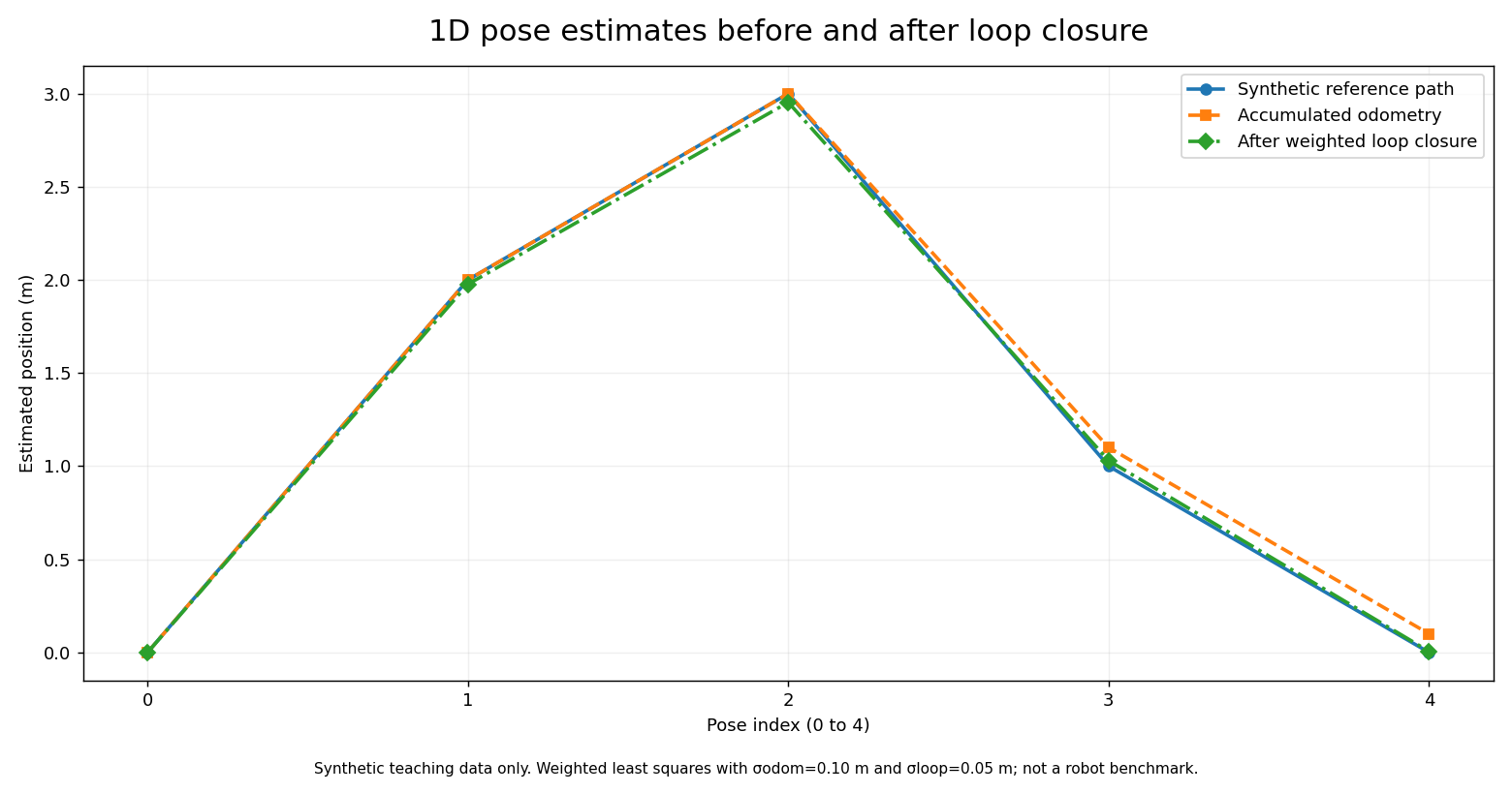
An instructive variation is to increase the loop closure’s assumed standard deviation from 0.05 m to 0.50 m, reducing its influence relative to odometry. The optimizer would then preserve more of the original drift. Conversely, making a false loop closure overly confident may distort many poses. Engineers should never treat a loop match’s score as automatically calibrated covariance without validation.

From a Linear Teaching Model to Real Graph-Based SLAM

Real mobile-robot SLAM includes orientation, sensor calibration and timestamping. A front end extracts relative-motion and possible loop constraints from encoders, inertial measurements, camera features or range scans. A back end optimizes accepted constraints. For example, two nearby-looking LiDAR scans may come from different locations with similar walls. A front end should verify a plausible geometric transform, useful overlap and consistency with other sensors before sending an edge to the back end.

When optimizing a nonlinear graph, a good initial trajectory estimate helps solvers converge to a meaningful local solution. Robust loss functions can reduce the influence of some outlier factors, but they do not guarantee recovery from a severely wrong loop closure. Some systems use switchable constraints, consistency checks, or separate place-recognition thresholds. Every choice trades runtime, accuracy, memory and failure behavior.

GTSAM offers batch nonlinear optimization and incremental approaches. ROS SLAM Toolbox provides mapping and serialization around pose-graph operations; its maintainer documentation describes continuing to refine a saved pose graph. A production deployment must be evaluated on representative environments and sensors, with quantitative trajectory and map metrics measured against independently obtained references.

Cyrill Stachniss, “Graph-based SLAM using Pose Graphs,” university Mobile Robotics teaching lecture, published April 3, 2020. The University of Bonn’s open training page lists the lecture. The presentation explains the graph model and optimization; it is distinct from the synthetic one-dimensional worked calculation.

Practical Lab: Reproducing and Stress-Testing the Result

1. Run the Python example exactly as shown and copy the five optimized positions. Check the return code and numerical output.
2. Repeat the run with all four odometry values unchanged but replace the loop-observation noise standard deviation 0.05 m with 0.50 m. Report how the final position changes and explain why.
3. Deliberately change the loop measurement from zero to +1.5 m and keep its high confidence. Observe whether the optimized path becomes less consistent with the known synthetic reference. Label that result a false-loop-closure failure example, not an actual SLAM attack.
4. Explain why the expected path RMSE here can be calculated only because the synthetic reference trajectory is known. A deployed robot usually lacks perfectly known ground truth.
5. Read the GTSAM Pose2 example, identifying the prior, consecutive relative-pose measurements, loop closure and optimization call. Document which items are new relative to the one-dimensional model.

Diagnostic Checklist and Failure Modes

• Odometry drift: compare predicted motion with independently observed positions, inspect wheel slip, encoder scaling and inertial bias; do not disguise a sensor fault by aggressive graph weighting.
• False place recognition: examine whether two visually similar locations were mistakenly equated, especially in repeating rows of shelves or corridors.
• Frame inconsistency: check the configured relationships among map, odom, base_link and the sensor frame using documented ROS tooling. Avoid mixing coordinates from different timestamps.
• Poor initialization: nonlinear optimization may settle at a poor local minimum when the starting pose guesses are severely inconsistent.
• Unanchored graph: gauge freedom can produce a rank-deficient system and nonunique global pose; use an appropriate prior or fixed reference.
• Unrealistic covariance: a small variance is not synonymous with trustworthy data, and tuning should reflect empirically validated sensor error.
• Latency and compute load: frequent graph updates may consume CPU and memory; record map size, pose count, processor, latency and actual error metrics before drawing performance conclusions.
• Map integrity: a numerically lower optimization objective is not proof of a correct map if the input constraints are wrong.

Safety, Deployment and Engineering Judgment

Robot autonomy must never be enabled on a real platform solely because a synthetic optimization script behaves correctly. Commissioning requires separately verified localization, emergency-stop and safeguarding behavior, localization-loss responses, speed limits, obstacle detection and facility operating procedures. Simulated mapping tutorials do not override the robot manufacturer’s safety manual. For a practical deployment, begin with logged sensor data or an approved simulation, then validate changes using a controlled testing plan.

Read OSRTC.016 on encoder and tracking-frame diagnostics for upstream motion errors, and OSREC.006 on feedback control for downstream motion control. An excellent map does not automatically create a safe navigation controller.

Knowledge Check and Answers

1. What is a loop closure? A verified measurement relating a later robot pose to a previously visited pose or location.
2. Why can a loop closure affect older poses? The optimizer jointly adjusts graph variables to reconcile multiple constraints rather than correcting one reading in isolation.
3. What does a factor express? A probabilistic or weighted relationship involving one or more unknown quantities, such as a prior or relative motion.
4. What is the final odometry estimate in the example? +0.10 m relative to the anchored origin.
5. What is the optimized final estimate? About +0.005882 m under the stated weight assumptions.
6. What changed in the error metric? Synthetic reference RMSE decreased from approximately 0.063246 m to 0.027084 m.
7. Why is a false loop closure dangerous? It can pull multiple poses toward an incorrect alignment and corrupt the reconstructed trajectory and map.
8. Why is a fixed first pose useful? It removes an otherwise arbitrary global translation/rotation freedom in relative-only pose estimation.
9. Is this Python example a real robot benchmark? No. It is a reproducible linear least-squares exercise with invented measurement data.

Primary Educational References

Open-source and educational references: GTSAM — Pose2 SLAM Example; GTSAM — Factor Graphs and a Hands-on Introduction; ROS 2 SLAM Toolbox package; Navigation2 — Mapping and Localization setup; StachnissLab / University of Bonn — Online Mobile Robotics Lectures; and MathWorks — Autonomous Navigation educational video series. The original graph-optimization model and numeric output were verified with a Python/NumPy calculation on November 7, 2026. Video titles, publishers and URLs were checked, but playback requires a separate player test.

Conclusion

Pose-graph optimization turns a sequence of uncertain local measurements into a globally more consistent trajectory when valid constraints tie past and present observations together. A defensible SLAM system distinguishes measured evidence, assumed noise, data association, the numerical solution and final physical validation. The lesson’s small worked example makes the mathematics transparent without pretending to establish performance on real-world hardware.

Editor’s Note: OSREC.014 follows published OSREC.013. The Python calculation and line chart use intentionally synthetic data and have been numerically checked, not measured on a robot. The featured 1200 × 630 image is original conceptual editorial artwork, not a documentary photograph. The in-story ROS image is a genuine official software documentation screenshot. No custom conceptual schematics or diagrams were produced. Educational video publishers and IDs were verified; live player rendering and playback are assessed separately.

Mobile scanning: view the article on another screen and scan the QR code using a compatible Bitcoin wallet, or import the saved QR image if your wallet supports that workflow. Confirm the recipient and the 5,000-sat amount before authorizing a transaction.

We volunteer daily to ensure the information on this platform is Verifiably True. If you would like to support the research, please scan the QR code.

BitcoinVersus.tech publishes independent technical education and journalism. No robotics safety certification or real-hardware performance test is implied.